38  Feedback Through Nodal Attribute Changes

This next tutorial will briefly demonstrate how changes to nodal attributes over time are another mechanism that results in feedback between the epidemic system and the dynamic network structure. In the context of diseases like HIV, partnership selection and activity level may vary based on disease status (more specifically, diagnosed disease status but we’ll ignore that complication in this model). Because disease status can change over time, any network model that references the disease status attribute must then be resimulated when the nodal attributes change. And these nodal attributes for disease status change as a function of the infections that result from the network structure. Therefore, the epidemic and the network feed back on each other. Unlike the previous demography tutorial, the population size stays fixed here: the feedback runs through a changing nodal attribute (disease status) rather than through arrivals and departures. This tutorial will walk through the parameterization and implications of this model.

NoteThe feedback loop in this model

Every network model so far has run in one direction: the network shapes the epidemic. This tutorial closes the loop. Disease status is now a term in the network model (through nodefactor and nodematch on status), so the network is no longer fixed, it is redrawn from the current distribution of statuses at every step.

That makes a two-way system:

• the network drives the epidemic: who partners with whom determines who gets infected, and
• the epidemic drives the network: each new infection flips a node’s status, which changes that node’s partnering, which changes the network the next infections run on.

The signature of this loop, and the thing to watch for in the results, is that the network statistics no longer hold flat at their targets. They move, because the population they describe is itself moving.

Note

Download the R script to follow along with this tutorial here.

38.1 Network Model

First, we will set up our network and then calculate our target statistics under the parameterization that people with infection have a lower mean degree than those without infection. This may be a function of behavioral change following disease diagnosis, which is commonly observed for HIV. We are not yet considering how they match up.

# Set a seed so the random infection assignment below (and the
# stochastic simulations that follow) reproduce the values shown here.
set.seed(12345)

n <- 500
nw <- network_initialize(n)

38.1.1 Parameterization

The initial prevalence in the network will be 20%. Note that we need to specify a vertex attribute, which must be called status, for this model. This is another “special” attribute on the network, like group, that is treated differently from any other named attribute. That is because status is the main attribute within netsim that keeps track of the individual disease status. We need to initialize the network like this with status as an individual attribute specifically because it will be a term within our TERGM; therefore, we will not randomly set the infected number with init.net as we have in previous tutorials.

NoteThe special status attribute

Disease status must live in a vertex attribute named exactly status. Like group, it is a special attribute that netsim reads and updates internally: it is how the model tracks who is infected. Because status is both set on the network and used as a TERGM term here, we seed the initial infections by hand rather than through init.net, and later hand netsim an empty init.net() placeholder.

Here, we assign exactly 100 nodes as infected, and randomly select which nodes those will be.

prev <- 0.2
infIds <- sample(1:n, n*prev)
nw <- set_vertex_attribute(nw, "status", "s")
nw <- set_vertex_attribute(nw, "status", "i", infIds)
get_vertex_attribute(nw, "status")

  [1] "s" "s" "s" "s" "i" "s" "i" "s" "s" "s" "s" "i" "i" "i" "s" "i" "s" "s"
 [19] "s" "s" "s" "s" "i" "s" "i" "s" "s" "s" "s" "s" "s" "s" "s" "i" "s" "i"
 [37] "s" "i" "s" "i" "s" "i" "s" "s" "s" "i" "s" "s" "s" "s" "i" "s" "s" "s"
 [55] "i" "i" "s" "i" "s" "i" "s" "i" "s" "s" "s" "s" "i" "i" "s" "s" "s" "s"
 [73] "s" "i" "i" "s" "s" "s" "s" "i" "s" "s" "s" "s" "s" "i" "s" "s" "s" "i"
 [91] "i" "s" "i" "s" "s" "s" "s" "s" "s" "s" "s" "s" "i" "s" "s" "i" "s" "s"
[109] "i" "s" "s" "s" "s" "s" "s" "i" "s" "s" "s" "s" "s" "s" "i" "i" "s" "s"
[127] "s" "s" "s" "s" "s" "s" "s" "s" "s" "s" "i" "s" "s" "s" "i" "i" "s" "s"
[145] "i" "s" "s" "i" "s" "s" "s" "i" "s" "i" "s" "s" "s" "s" "s" "s" "s" "s"
[163] "i" "s" "i" "i" "s" "s" "s" "s" "s" "s" "s" "s" "s" "s" "s" "s" "s" "s"
[181] "s" "s" "s" "s" "s" "s" "s" "s" "s" "s" "s" "i" "s" "s" "s" "s" "s" "s"
[199] "s" "s" "s" "s" "s" "s" "s" "s" "s" "i" "s" "s" "i" "i" "s" "i" "s" "i"
[217] "s" "i" "s" "i" "s" "s" "i" "s" "s" "s" "s" "s" "i" "s" "s" "i" "s" "i"
[235] "s" "s" "s" "s" "s" "s" "s" "s" "s" "s" "s" "s" "s" "s" "s" "s" "s" "i"
[253] "s" "s" "i" "s" "i" "i" "i" "s" "s" "s" "s" "s" "s" "i" "i" "s" "s" "s"
[271] "i" "s" "s" "s" "s" "s" "s" "s" "s" "s" "s" "s" "s" "s" "s" "i" "s" "i"
[289] "s" "s" "s" "s" "s" "i" "s" "s" "s" "s" "s" "s" "s" "s" "s" "s" "i" "s"
[307] "s" "s" "s" "s" "s" "s" "s" "i" "s" "s" "s" "s" "s" "s" "s" "s" "i" "s"
[325] "s" "s" "s" "i" "s" "s" "s" "s" "s" "s" "s" "s" "s" "s" "s" "s" "s" "s"
[343] "s" "s" "s" "s" "s" "s" "s" "i" "i" "i" "s" "i" "i" "s" "s" "s" "s" "s"
[361] "i" "s" "i" "s" "s" "s" "s" "s" "s" "s" "s" "s" "s" "s" "i" "s" "i" "s"
[379] "s" "s" "s" "s" "i" "s" "s" "s" "s" "s" "i" "s" "i" "s" "i" "s" "s" "i"
[397] "s" "s" "i" "s" "s" "s" "s" "s" "s" "s" "s" "s" "s" "s" "s" "s" "s" "s"
[415] "s" "i" "s" "s" "s" "s" "s" "s" "i" "s" "s" "s" "s" "i" "s" "s" "s" "s"
[433] "i" "i" "i" "s" "i" "s" "s" "s" "s" "s" "s" "s" "s" "s" "s" "i" "i" "s"
[451] "s" "s" "s" "s" "s" "s" "s" "s" "s" "i" "s" "s" "s" "s" "i" "s" "s" "s"
[469] "s" "s" "s" "s" "s" "s" "s" "s" "s" "s" "s" "s" "s" "i" "s" "s" "s" "s"
[487] "s" "s" "s" "s" "s" "i" "s" "s" "s" "s" "s" "s" "s" "s"

A nodefactor term will allow the mean degree of the infected persons to differ from that of susceptible persons. In the previous tutorial, we calculated the nodefactor target statistic as the mean degree of a group times the size of the group. Another way of expressing that is a count of the number of times a member of a group, here an infected person or susceptible person, shows up in an edge. And this is just the group mean degree times the group size; here, the group size is defined by the disease prevalence, prev, variable specified above.

mean.deg.inf <- 0.3
inedges.inf <- mean.deg.inf * n * prev
inedges.inf

[1] 30

mean.deg.sus <- 0.8
inedges.sus <- mean.deg.sus * n * (1 - prev)
inedges.sus

[1] 320

The number of edges then is the sum of these two nodefactor statistics divided by 2 (because nodefactor is an expression of nodes).

edges <- (inedges.inf + inedges.sus)/2
edges

[1] 175

Next, let’s move on to parameterizing mixing by disease status. In this theoretically parameterized model, here again it is helpful to think about this in terms of what the expected statistic would be in the absence of any preferential or assortative mixing. That is, what is the value of the nodematch target statistic under a proportional (random) mixing model? For equally sized groups with the same mean degree, random mixing would put about half of all ties within-group. It gets more complicated here because the groups are of different sizes and have different activity levels. There are different ways to find this solution.

NoteWhat “no preference” looks like when groups differ

Before we can call anything serosorting, we need the baseline it is measured against: what would the within-status share of ties be with no behavioral preference at all? The tempting guess is 50%, but that holds only when the groups are the same size and equally active. Here susceptibles are both more numerous (80% of people) and more active (higher mean degree), so they fill a much larger share of relationship slots than infecteds do. By chance alone, then, most ties will be susceptible-susceptible.

The two calculations below both find that chance baseline, one exact (Hardy-Weinberg) and one by simulation, and both count relationship slots rather than people. The answer, 84%, is the bar: only within-status ties above 84% reflect a real preference, which is why the model will target 91% rather than 84%. That 84% is a proportional-mixing benchmark, the within-status share expected under random mixing, not an exact identity that any single finite network satisfies. A realized network scatters around it, which is exactly what the simulation-based calculation below makes visible.

The exact solution: from population genetics, the Hardy-Weinberg Principle. The idea maps directly onto our problem: treat each end (or “stub”) of a partnership as drawing a status at random, in proportion to how many relationship slots each status group occupies. The chance that a partnership is within-status is then the chance both ends are susceptible plus the chance both are infected, exactly the Hardy-Weinberg “homozygote” frequencies. The relevant proportions are of relationship slots, not of persons: because susceptibles here have a higher mean degree, they occupy a larger share of slots than their headcount alone would suggest. The code below builds the two-by-two table of pair probabilities (an S-S, I-I, or S-I pair); the matched (within-status) fraction is the diagonal, the sum of the S-S and I-I probabilities.

# Fraction of relationship slots (edge stubs) occupied by susceptibles
# vs. infecteds. inedges.sus counts susceptible stubs and edges * 2 is
# the total number of stubs. This share is activity-weighted, so it is
# not the same as the fraction of persons who are susceptible.
p.sus <- inedges.sus / (edges * 2)
p.inf <- 1 - p.sus

# Under random (proportional) mixing, the pair probabilities follow
# Hardy-Weinberg: both susceptible, one of each, or both infected.
pr.ss <- p.sus^2
pr.si <- 2 * p.sus * p.inf
pr.ii <- p.inf^2

# The matched (within-status) fraction is the diagonal of the table.
round(pr.ss + pr.ii, 3)

[1] 0.843

A simulation-based solution: we estimate an ERGM in which there is no nodematch term but heterogeneity in activity, then simulate from that fitted model to calculate the expected number of matched edges. The proportion of matched edges is that number over the total edges.

fit <- netest(nw,
              formation = ~edges + nodefactor("status"),
              target.stats = c(edges, inedges.sus),
              coef.diss = dissolution_coefs(~offset(edges), duration = 1))
sim <- netdx(fit, dynamic = FALSE, nsims = 1e4,
             nwstats.formula = ~edges + nodematch("status"))

Network Diagnostics
-----------------------
- Simulating 10000 networks
- Calculating formation statistics

stats <- get_nwstats(sim)
head(stats)

  sim edges nodefactor.status.s nodematch.status
1   1   185                 331              146
2   2   169                 303              134
3   3   182                 339              157
4   4   185                 337              154
5   5   167                 311              144
6   6   197                 361              170

round(mean(stats$nodematch.status/stats$edges), 3)

[1] 0.843

The main substantive finding here is that 84% of relations are expected to be within the same disease status group under proportional mixing, even without a behavioral preference for assortative mixing. This is because susceptible persons are a larger group in the population, and have more relationships per-capita.

Let us now imagine that there are in fact slightly more within-group ties than expected by chance:

nmatch <- edges * 0.91

38.1.2 Estimation

This tutorial will compare two models to assess the impact of behavior driven by disease status on epidemic trajectories:

• Model 1 features two forms of seroadaptive behavior: a difference in activity level by disease status (infected people partner less), and assortative matching on status. That second piece, the tendency to partner preferentially with others of the same status, is serosorting in the strict sense. Throughout this tutorial we reserve “serosorting” for that matching mechanism, and use “seroadaptive behavior” for the combined activity-and-matching response.
• Model 2 has neither, so is just a Bernoulli model with same mean degree as Model 1.

38.1.2.1 Model 1

The seroadaptive network model includes terms for both the number of times susceptible persons show up in an edge (the activity difference), as well as the number of node-matched edges overall (the serosorting). It is unnecessary to specify a nodefactor term for the infected persons because that count is a function of the total edges and the nodefactor term for the susceptible persons (the base level is always the first in alphabetical or numerical order, so “i” for our status variable level in this case). The average partnership duration in both models will be 50 weeks.

formation <- ~edges + nodefactor("status") + nodematch("status")
target.stats <- c(edges, inedges.sus, nmatch)

coef.diss <- dissolution_coefs(dissolution = ~offset(edges), duration = 50)

est <- netest(nw, formation, target.stats, coef.diss)

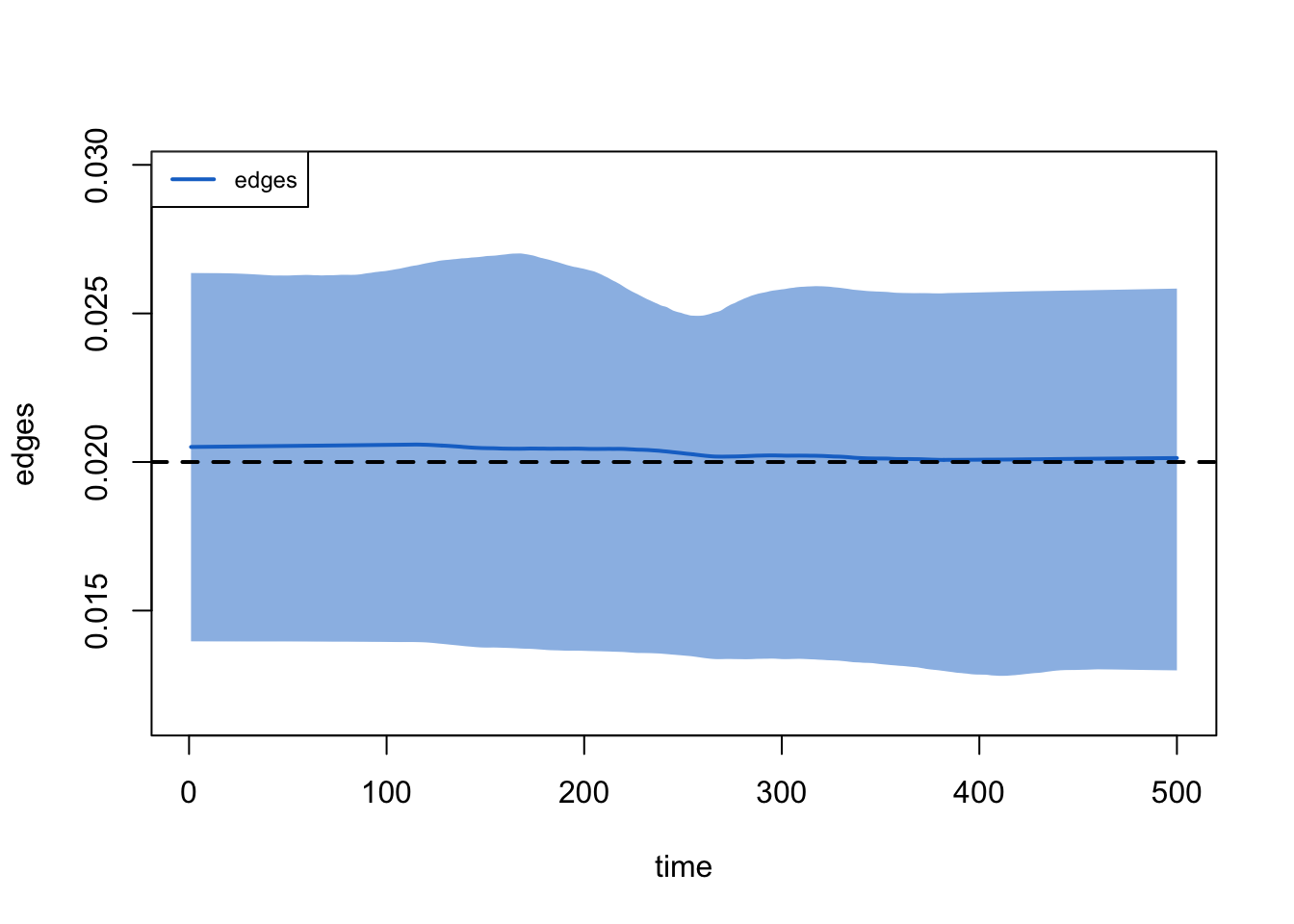
We run the network diagnostics on the model.

dx <- netdx(est, nsims = 10, nsteps = 1000, ncores = 5,
            nwstats.formula = ~edges + 
                               meandeg + 
                               nodefactor("status", levels = NULL) + 
                               nodematch("status"), verbose = FALSE)
dx

EpiModel Network Diagnostics
=======================
Diagnostic Method: Dynamic
Simulations: 10
Time Steps per Sim: 1000

Formation Diagnostics
----------------------- 
                    Target Sim Mean Pct Diff Sim SE Z Score SD(Sim Means)
edges               175.00  175.155    0.088  1.024   0.151         4.571
meandeg                 NA    0.701       NA  0.004      NA         0.018
nodefactor.status.i     NA   30.374       NA  0.596      NA         1.396
nodefactor.status.s 320.00  319.935   -0.020  1.938  -0.033         8.619
nodematch.status    159.25  159.190   -0.038  0.986  -0.061         4.377
                    SD(Statistic)
edges                      12.578
meandeg                     0.050
nodefactor.status.i         6.621
nodefactor.status.s        23.922
nodematch.status           12.151

Duration Diagnostics
----------------------- 
      Target Sim Mean Pct Diff Sim SE Z Score SD(Sim Means) SD(Statistic)
edges     50   49.785    -0.43  0.318  -0.677         0.861         3.567

Dissolution Diagnostics
----------------------- 
      Target Sim Mean Pct Diff Sim SE Z Score SD(Sim Means) SD(Statistic)
edges   0.02     0.02    0.234      0   0.443             0         0.011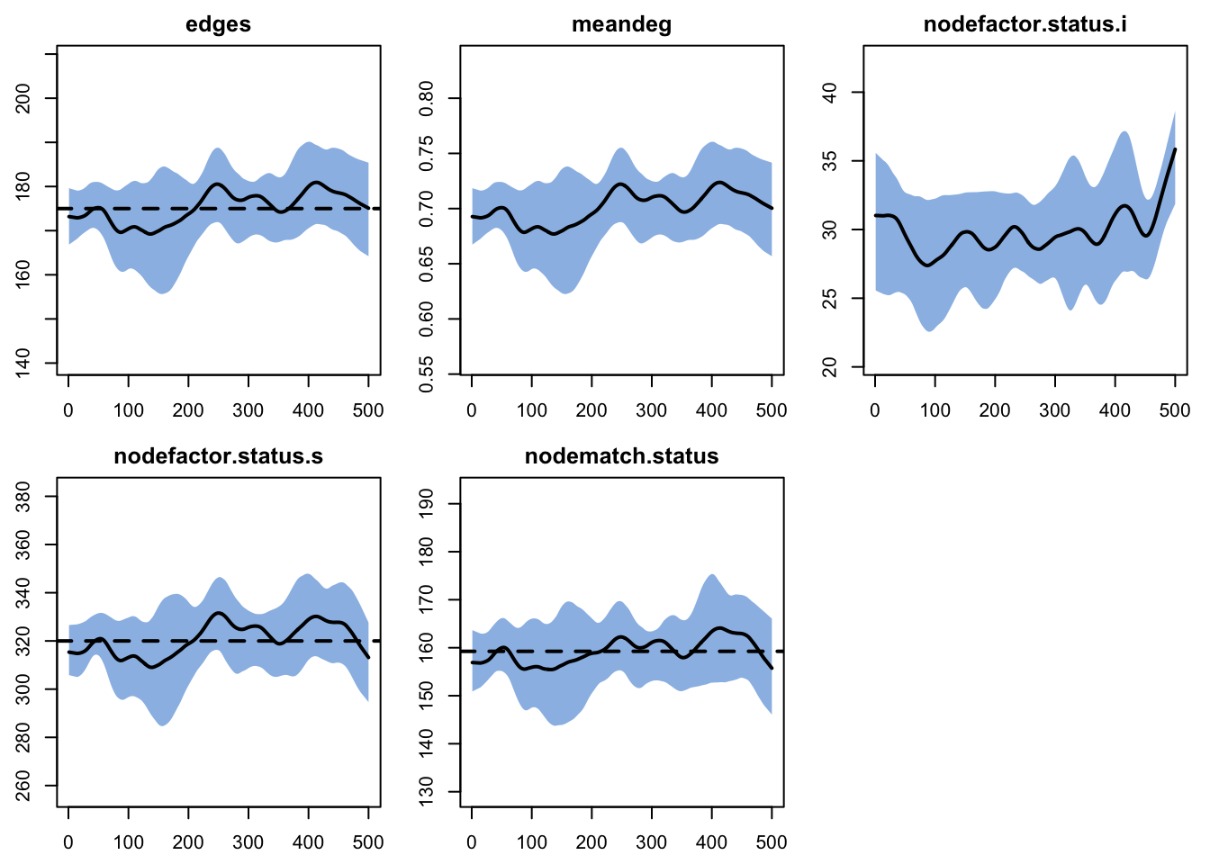

plot(dx)

plot(dx, type = "dissolution")

38.1.2.2 Model 2

The second model will include only an edges term, so no seroadaptive behavior but same amount of activity among nodes. We are recycling the nw object with the status attribute set from above.

est2 <- netest(nw, formation = ~edges, target.stats = edges, coef.diss)

After estimation, the diagnostics here look fine too. Compare the nodefactor and nodematch simulations here to those in the Model 1 diagnostics: more edges for infected persons, and more discordant edges (partnerships between one infected and one susceptible node).

dx2 <- netdx(est2, nsims = 10, nsteps = 1000, ncores = 5,
             nwstats.formula = ~edges + 
                                meandeg + 
                                nodefactor("status", levels = NULL) + 
                                nodematch("status"), verbose = FALSE)
dx2

EpiModel Network Diagnostics
=======================
Diagnostic Method: Dynamic
Simulations: 10
Time Steps per Sim: 1000

Formation Diagnostics
----------------------- 
                    Target Sim Mean Pct Diff Sim SE Z Score SD(Sim Means)
edges                  175  174.863   -0.079  1.257  -0.109         4.497
meandeg                 NA    0.699       NA  0.005      NA         0.018
nodefactor.status.i     NA   71.390       NA  0.850      NA         3.642
nodefactor.status.s     NA  278.335       NA  2.065      NA         6.481
nodematch.status        NA  117.765       NA  0.949      NA         2.426
                    SD(Statistic)
edges                      13.622
meandeg                     0.054
nodefactor.status.i         9.713
nodefactor.status.s        22.597
nodematch.status           10.548

Duration Diagnostics
----------------------- 
      Target Sim Mean Pct Diff Sim SE Z Score SD(Sim Means) SD(Statistic)
edges     50    50.29    0.581  0.369   0.786         1.213         4.021

Dissolution Diagnostics
----------------------- 
      Target Sim Mean Pct Diff Sim SE Z Score SD(Sim Means) SD(Statistic)
edges   0.02     0.02    0.038      0   0.074             0         0.011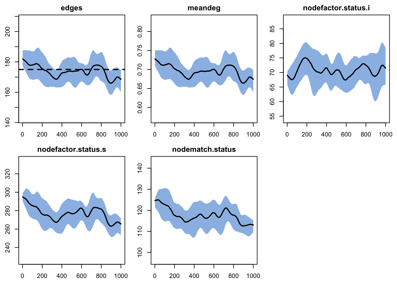

plot(dx2)

38.2 Epidemic Model

For the epidemic model, we will simulate an SI disease, with our two counterfactual network models. The first model will use the seroadaptive network model, and the second will be the random Bernoulli model.

38.2.1 Model 1

The model will only include one named parameter, for the transmission probability per contact.

param <- param.net(inf.prob = 0.03)

The initial conditions are now passed through to the epidemic model not through init.net as with previous examples, but through the netest object that contains the original starting network with the vertex attributes for status. However, because netsim will still be expecting an initial conditions list, we need to create an empty object as a placeholder.

init <- init.net()

For the control settings, we monitor the same network statistics as we did in the network diagnostics above. The resimulate.network argument must be set to TRUE because the network needs to be updated at each time step. In this model, we will use the tergmLite approach since we do not need to monitor individual-level network histories.

control <- control.net(type = "SI", nsteps = 500, nsims = 5, ncores = 5,
                       resimulate.network = TRUE, tergmLite = TRUE,
                       nwstats.formula = ~edges + 
                                          meandeg + 
                                          nodefactor("status", levels = NULL) + 
                                          nodematch("status"))

Here, we run the model. We will return to it to compare output later.

sim <- netsim(est, param, init, control)

38.2.2 Model 2

The second model includes the same epidemic parameters as Model 1, so all that we need to change is the first parameter for the different network object.

sim2 <- netsim(est2, param, init, control)

38.2.3 Results

Here we’ll look at the epidemic results first and then the network diagnostics, because the network statistics will be a function of the epidemiology.

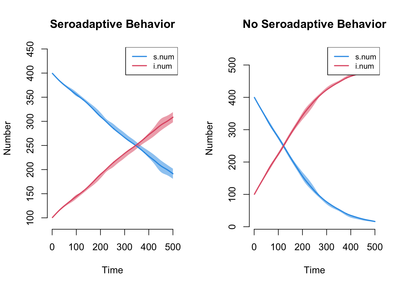
Here we see that the seroadaptive model grows much less quickly than the random model. The reasons are that nodes lower their mean degree upon infection, and therefore have fewer partners over time (the activity difference). They also tend to preferentially partner with other infecteds (serosorting).

par(mfrow = c(1,2))
plot(sim, main = "Seroadaptive Behavior")
plot(sim2, main = "No Seroadaptive Behavior")

Another method to show the relative difference is to plot the two epidemic trajectories together. This requires a custom legend.

par(mfrow = c(1,1))
plot(sim, y = "i.num", popfrac = TRUE, sim.lines = FALSE, qnts = 1)
plot(sim2, y = "i.num", popfrac = TRUE, sim.lines = FALSE, qnts = 1, 
     mean.col = 2, qnts.col = 2, add = TRUE)
legend("topleft", c("Seroadaptive", "Non-seroadaptive"), lty = 1, lwd = 3,
       col = c(4, 2), cex = 0.9, bty = "n")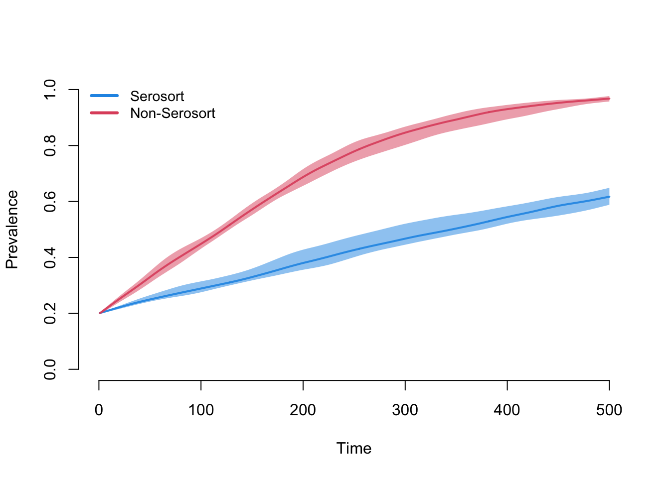

Now, here are the network statistics that we monitored in Model 1. In contrast to our previous tutorials, where we expected stochastic variation around the targets to be preserved over time, here every network statistic varies.

NoteHere, drifting statistics are the right answer

In every earlier tutorial a correct model held its network statistics flat at their targets, and drift was a warning sign. Here it is the opposite: the drift is the result. The targets describe the population at the start, when prevalence is 20%. As the epidemic runs, prevalence climbs to about 50% by the end of the 500-step run (in an SI model with no recovery it would keep rising past that if we simulated longer), and because infected people partner less, the whole population partners less: mean degree falls, edges fall, and the who-partners-with-whom mix shifts. Nothing is misbehaving; the model is faithfully passing the epidemic’s changes back into the network.

What the model actually holds fixed is not a count but the conditional log-odds (the coefficient) of a susceptible appearing in a tie. The realized counts are free to follow the changing population, which is exactly what feedback means.

plot(sim, type = "formation", qnts = FALSE, sim.lines = TRUE)

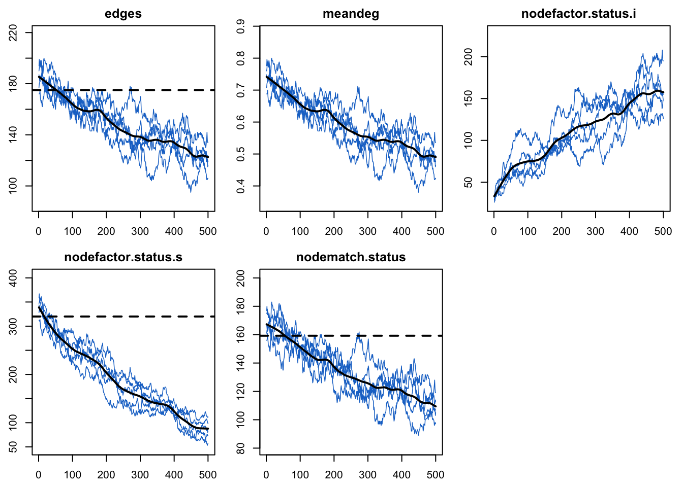
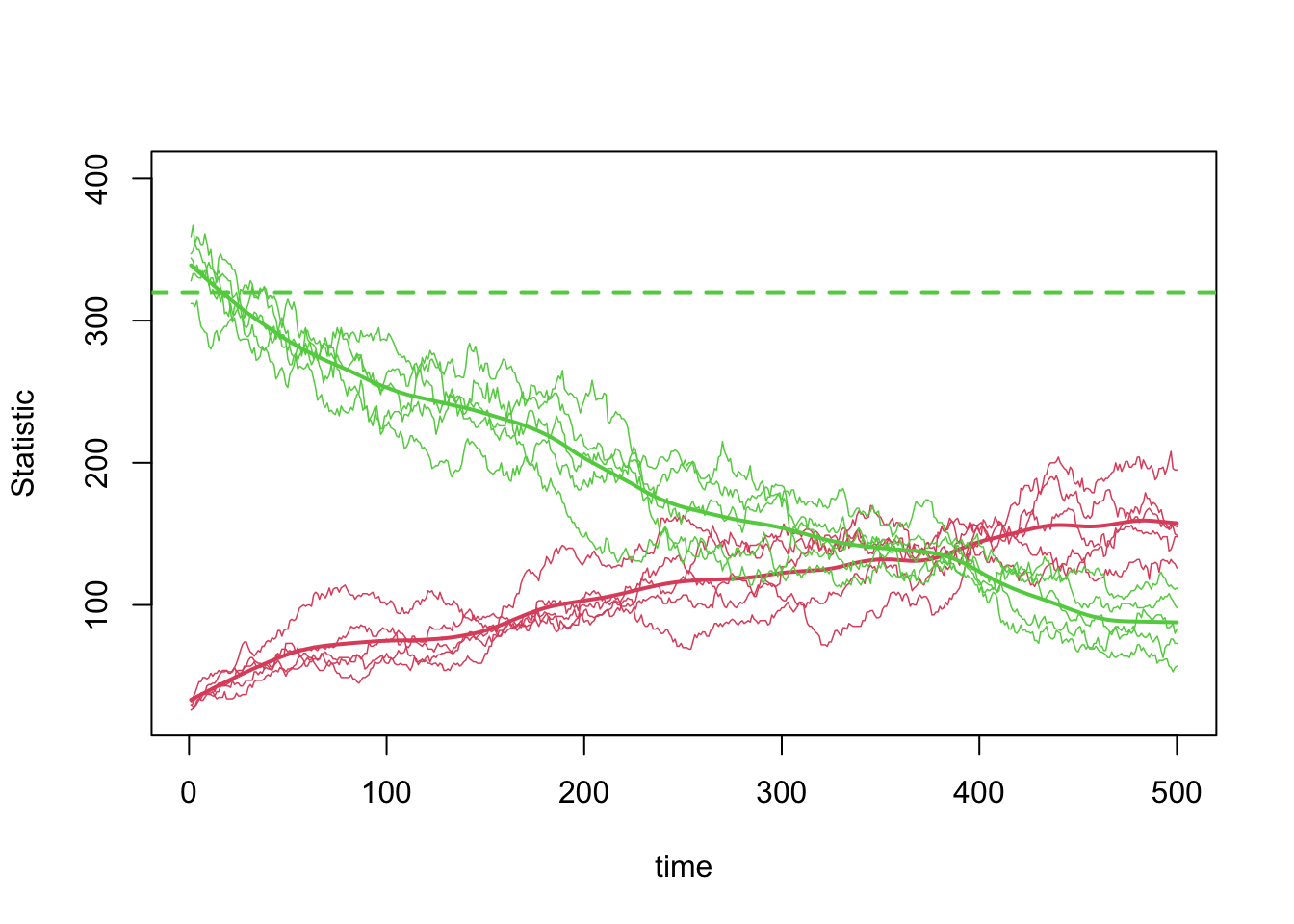
Notice first that the nodefactor statistics are moving in opposite directions: as the prevalence of disease increases from 20% to approximately 50% at time 500, the number of infected nodes in an edge increases. The quantity preserved is not the raw nodefactor count that we set as a target (the 320 susceptible node-appearances); rather, it is the log-odds of a susceptible node appearing in an edge, conditional on the other terms in the model.

plot(sim, type = "formation", qnts = FALSE, sim.lines = TRUE,
     stats = c("nodefactor.status.s", 
               "nodefactor.status.i"))

Second, note that the total edges and node-matched edges decline over time. This plot shows those two statistics from one simulation only for clarity. Ordinarily netsim’s network-size correction preserves mean degree even when the population size changes. In this model the population size never changes, so that correction is not what is happening here.

plot(sim, type = "formation", 
     stats = c("edges", "nodematch.status"), 
     qnts = FALSE, sims = 1, sim.lwd = 2)

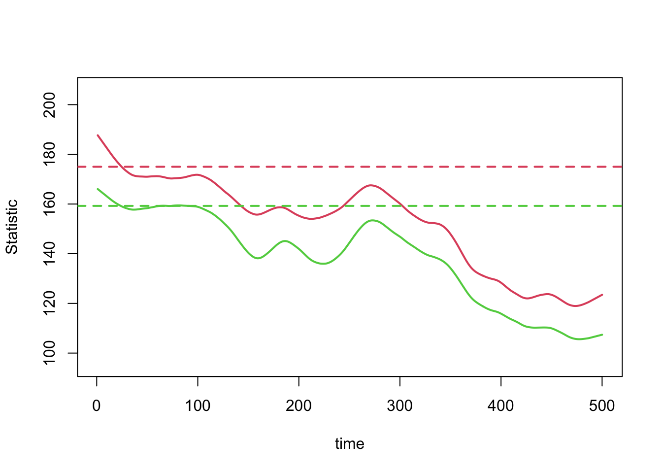
Instead, the edges and mean degree are shrinking because the number of infected nodes in the network is steadily increasing, which draws the node-match statistic lower since there are fewer susceptible-susceptible pairs available. Note that the fixed 0.91 ratio we imposed applies only to the initial targets, not to these realized series: under feedback both statistics are free to drift, and here they happen to fall together because the same force (rising prevalence and the resulting decline in overall partnering) drives both down. This is why the raw nodematch count is the wrong thing to watch for whether the serosorting preference is holding: the count moves as the status composition moves, even if the behavioral preference itself does not change. The quantity that isolates preference is the matched-edge fraction measured against the proportional-mixing benchmark for the current composition, the p^2 + q^2 calculation above recomputed at the current prevalence, not the raw count and not the initial 0.91 target.

After looking at so many models where the target statistics were preserved throughout the simulation, this may seem like odd or undesirable behavior here. If it does, think about the main assumption we began with: persons who are infected tend to have lower rates of partnering than persons who are not infected. Perhaps this is because they are ill, or because they are trying to protect others. If this is the case, then what should we expect to happen to the overall rate of partnering as the proportion of persons who are infected increases? Presumably it should go down, which is precisely what we see.

This behavior does mean that it can be difficult to tease apart the different contributions of the seroadaptive response to the disease dynamics that we see. How much of the seroadaptive response’s effect on lowering transmission came from the overall partner reductions among infected persons, and how much came from serosorting, the homophily effect where infected persons partner with each other relatively more? Although we included both in our model (through the nodefactor and nodematch terms, respectively), one could easily consider intermediate models that only included one term or the other, and then compare the results of each to the two models we already considered. We would then have a sense of the individual effects of each of these behavioral components, as well as their combined effect. Is the latter additive, less than additive, or more than additive (i.e., synergistic)?