42  Adding a Latent Stage to Make an SEIR Model

EpiModel includes an integrated SIR model, but here we show how to model an SEIR disease, one with a latent (exposed) stage between infection and infectiousness, as many respiratory infections have. The E compartment is an exposed state in which a person has been infected but is not infectious to others. Some infectious diseases have this latent non-infectious stage, and in general it provides a general framework for transmission risk that is dependent on one’s stage of disease progression. The parameters used below are stylized to demonstrate the extension API clearly rather than calibrated to any specific pathogen, and the time step is an abstract unit; for a real analysis you would substitute published estimates and fix the time step (for example, a day or a week).

Note

This tutorial has two R scripts you should download: a primary script containing the code below and a separate module script. Download both and put them in the same working directory.

NoteBuild it once to learn the API, reuse the maintained copy

We build this SEIR module by hand because writing one module yourself is the fastest way to internalize the extension API. The same model, parameterized to provide both SEIR and SEIRS from a single module, is maintained as a Gallery example: SEIR/SEIRS: Adding an Exposed State. That is the copy you would actually reuse and extend, and the lab works directly with it. The get_/set_ accessors and control.net settings used below are documented in full in the EpiModel package vignettes at epimodel.org.

42.1 Setup

First start by loading EpiModel and clearing your global environment.

library(EpiModel)
rm(list = ls())
set.seed(12345)

42.2 EpiModel Model Extensions

42.2.1 Conceptualization

The first step to any EpiModel extension model is to conceptually identify what new functionality, above and beyond the built-in models, is desired and where that functionality should be added. There are often many “right” answers to these questions, and this aspect is only learned over time. But in general, it is helpful to map out a model extension on a state/flow diagram to pinpoint where the additions should be concentrated.

42.2.1.1 SIR Module Set

In this particular model, we will be adding a new disease state that occurs in between the susceptible disease state and an infectious disease state in an SIR model. The standard, built-in SIR model in EpiModel uses a set of modules (elements of the model), each with its own associated function (the realization of those elements in code). To ground the discussion, let’s fit and run a basic built-in SIR model and print the result.

nw <- network_initialize(n = 100)
formation <- ~edges
target.stats <- 50
coef.diss <- dissolution_coefs(dissolution = ~offset(edges), duration = 20)
est1 <- netest(nw, formation, target.stats, coef.diss, verbose = FALSE)
param <- param.net(inf.prob = 0.3, rec.rate = 0.1)
init <- init.net(i.num = 10, r.num = 0)
control <- control.net(type = "SIR", nsteps = 25, nsims = 1, verbose = FALSE)
mod1 <- netsim(est1, param, init, control)
mod1

EpiModel Simulation
=======================
Model class: netsim

Simulation Summary
-----------------------
Model type: SIR
No. simulations: 1
No. time steps: 25
No. NW groups: 1

Fixed Parameters
---------------------------
inf.prob = 0.3
rec.rate = 0.1
act.rate = 1
groups = 1

Model Output
-----------------------
Variables: s.num i.num r.num num si.flow ir.flow
Networks: sim1
Transmissions: sim1

Formation Statistics
----------------------- 
      Target Sim Mean Pct Diff Sim SE Z Score SD(Sim Means) SD(Statistic)
edges     50    48.32    -3.36  3.822   -0.44            NA         6.115


Duration Statistics
----------------------- 
      Target Sim Mean Pct Diff Sim SE Z Score SD(Sim Means) SD(Statistic)
edges     20   18.105   -9.476  0.329  -5.757            NA         1.113

Dissolution Statistics
----------------------- 
      Target Sim Mean Pct Diff Sim SE Z Score SD(Sim Means) SD(Statistic)
edges   0.05     0.05    0.149  0.007   0.011            NA         0.034

Printing a built-in model reports its type, run settings, and the compartments and flows it tracked, but not the list of module functions: for a built-in model EpiModel selects those internally from type. Two things do expose the module set. The control.net argument list (below) names every module slot, and once we build our own extension model later in this tutorial (with type = NULL), printing it adds a Model Functions section that lists exactly the modules that ran.

42.2.1.2 Module Classes

This includes a series of modules, which we classify into Standard and Flexible modules as shown on the table below. Any modules may be modified, but standard modules are those that are typically not modified because they generalize the core internal processes for simulation object generation, network resimulation, and epidemic bookkeeping. Flexible modules, in contrast, are those that are likely necessary to modify for an EpiModel extension.

In the example above, we used all of these modules except the arrivals and departures modules because we had a closed population. In addition to these set of built-in modules, any user can add more modules to this set, depending on what is needed. Again, this involves some conceptualization of how to organize the model processes, including whether those processes are similar to the built-in modules or something new.

42.2.1.3 Modules vs. Functions

All modules have associated functions, and these are passed into the epidemic model run in netsim through control.net. Printing out the arguments for this function, you will see that each of the standard modules have default associated functions as inputs, and flexible modules have a default of NULL.

args(control.net)

function (type, nsteps, start = 1, nsims = 1, ncores = 1, resimulate.network = FALSE, 
    tergmLite = FALSE, cumulative.edgelist = FALSE, truncate.el.cuml = 0, 
    attr.rules, epi.by, initialize.FUN = initialize.net, resim_nets.FUN = resim_nets, 
    summary_nets.FUN = summary_nets, infection.FUN = NULL, recovery.FUN = NULL, 
    departures.FUN = NULL, arrivals.FUN = NULL, nwupdate.FUN = nwupdate.net, 
    prevalence.FUN = prevalence.net, verbose.FUN = verbose.net, 
    module.order = NULL, save.nwstats = TRUE, nwstats.formula = "formation", 
    save.transmat = TRUE, save.network, save.run = FALSE, save.cumulative.edgelist = FALSE, 
    save.other, verbose = TRUE, verbose.int = 1, skip.check = FALSE, 
    raw.output = FALSE, future.use.plan = FALSE, tergmLite.track.duration = FALSE, 
    set.control.ergm = control.simulate.formula(MCMC.burnin = 2e+05), 
    set.control.tergm = control.simulate.formula.tergm(MCMC.maxchanges = .Machine$integer.max), 
    save.diss.stats = TRUE, dat.updates = NULL, ...) 
NULL

For built-in models, EpiModel selects which modules are needed based on the model parameters and initial conditions. For each time step, the modules run in the order in which they are specified in the output here, which for a built-in model matches the order in which they are listed in control.net. Extension models add one wrinkle we will meet below: a module passed under a name that is not one of control.net’s own arguments is a user module, and EpiModel runs all user modules before all built-in ones, whatever order they were written in.

42.2.1.4 Built-in Functions as Templates

Any of the built-in functions associated with flexible modules are intended to be templates for user inspection and extension for research-level models. A built-in SIR model uses infection.net as its infection module. That function has a help page briefly describing what it does. And you can also inspect the function contents with:

View(infection.net)

We’ll use an edited down version of that function, with some additional explanation, below. In addition, the disease progression state transition within an SIR model (and an SIS model too) is handled by the recovery module, with an associated recovery.net function.

View(recovery.net)

We will use an edited down version of that function as a template for a new, more general disease progression module.

42.2.2 The EpiModel API

All EpiModel module functions have a set of shared design requirements. This set of requirements defines the EpiModel Application Programming Interface (API) for extension. The best way to learn this is through a concrete example like this, but here are the general API rules:

1. Each module has an associated R function, the general design of which is:

fx <- function(dat, at) {
  
  ## function processes that update dat
  
  return(dat)
}

The function takes an object called dat, which is the master data object passed around by netsim, performs some processes (e.g., infection, recovery, aging, interventions), updates the dat object, and then returns that object. The other input argument to each function must be at, which is a time step counter.

2. Data are stored on the dat object in a particular way: in sublists that are organized by category. The main categories of data to interact with include model inputs (parameters, initial conditions, and controls) from those three associated input functions; nodal attributes (e.g., an individual disease status for each person); and summary statistics (e.g., the disease prevalence at at time step). There are accessor functions for reading (these are the get_ functions) and writing (these are the set_ functions) to the dat object in the appropriate place.

3. The typical function design involves three steps: a) reading the relevant inputs from the dat object; b) performing some micro-level process on the nodes that is usually a function of fixed parameters and time-varying nodal attributes; c) writing the updated objects back on to the dat object.

Let’s see how this API works by extending our infection and recovery functions to transition an SIR model into an SEIR model.

42.2.3 Infection Module

The built-in infection module for an SIR model performs the following functions listed in the function below. The core process is determining which edges are eligible for a disease transmission to occur, and then randomly simulating that transmission process. Why is it necessary to update the infection function for an SEIR model? Because an SIR involves a transition between S and I disease statuses when a new infection occurs, but an SEIR model involves a transition between S and E disease statuses. It’s a small, but important change. Here’s the full modified function, with embedded comments. Note that we can use the browser function to run this function in debug mode by uncommenting the third line (we will demonstrate this).

infect <- function(dat, at) {

  ## Uncomment this to run environment interactively
  # browser()

  ## Attributes ##
  active <- get_attr(dat, "active")
  status <- get_attr(dat, "status")
  infTime <- get_attr(dat, "infTime")

  ## Parameters ##
  inf.prob <- get_param(dat, "inf.prob")
  act.rate <- get_param(dat, "act.rate")

  ## Find infected nodes ##
  idsInf <- which(active == 1 & status == "i")
  nActive <- sum(active == 1)
  nElig <- length(idsInf)

  ## Initialize default incidence at 0 ##
  nInf <- 0

  ## If any infected nodes, proceed with transmission ##
  if (nElig > 0 && nElig < nActive) {

    ## Look up discordant edgelist ##
    del <- discord_edgelist(dat, at)

    ## If any discordant pairs, proceed ##
    if (!(is.null(del))) {

      # Set parameters on discordant edgelist data frame
      del$transProb <- inf.prob
      del$actRate <- act.rate
      del$finalProb <- 1 - (1 - del$transProb)^del$actRate

      # Stochastic transmission process
      transmit <- rbinom(nrow(del), 1, del$finalProb)

      # Keep rows where transmission occurred
      del <- del[which(transmit == 1), ]

      # Look up new ids if any transmissions occurred
      idsNewInf <- unique(del$sus)
      nInf <- length(idsNewInf)

      # Set new attributes and transmission matrix
      if (nInf > 0) {
        status[idsNewInf] <- "e"
        infTime[idsNewInf] <- at
        dat <- set_attr(dat, "status", status)
        dat <- set_attr(dat, "infTime", infTime)

        dat <- set_transmat(dat, del, at)
  
      }
    }
  }

  ## Save summary statistic for S->E flow
  dat <- set_epi(dat, "se.flow", at, nInf)

  return(dat)
}

Each step is relatively self-explanatory with the comments, but we will run this interactively at the end of this tutorial to step through the updated data structures. Infection is one of the more complex processes because it involves a dyadic process (a contact between an S and I node). That involves a construction of a discordant edgelist; that is, a list of edges in which there is a disease discordant dyad.

The main point here is: we have made a change to the infection module function, and it consists of updating the disease status of a newly infected persons to "e" instead of "i". Additionally, we are tracking a new summary statistic, se.flow that tracks the size of the flow from S to E based on the number of new infected, nInf at the time step.

42.2.4 Progression Module

Next up is the disease progression module. Here, we have generalized the built-in recovery module function to handle two disease progression transitions after infection: E to I (latent to infectious stages) and I to R (infectious to recovered stages). Like many individual-level transitions, this involves flipping a weighted coin with rbinom: this performs a series of random Bernoulli draws based on the specified parameters. Here is the full model function.

progress <- function(dat, at) {

  ## Uncomment this to function environment interactively
  # browser()

  ## Attributes ##
  active <- get_attr(dat, "active")
  status <- get_attr(dat, "status")

  ## Parameters ##
  ei.rate <- get_param(dat, "ei.rate")
  ir.rate <- get_param(dat, "ir.rate")

  ## E to I progression process ##
  nInf <- 0
  idsEligInf <- which(active == 1 & status == "e")
  nEligInf <- length(idsEligInf)

  if (nEligInf > 0) {
    vecInf <- which(rbinom(nEligInf, 1, ei.rate) == 1)
    if (length(vecInf) > 0) {
      idsInf <- idsEligInf[vecInf]
      nInf <- length(idsInf)
      status[idsInf] <- "i"
    }
  }

  ## I to R progression process ##
  nRec <- 0
  idsEligRec <- which(active == 1 & status == "i")
  nEligRec <- length(idsEligRec)

  if (nEligRec > 0) {
    vecRec <- which(rbinom(nEligRec, 1, ir.rate) == 1)
    if (length(vecRec) > 0) {
      idsRec <- idsEligRec[vecRec]
      nRec <- length(idsRec)
      status[idsRec] <- "r"
    }
  }

  ## Write out updated status attribute ##
  dat <- set_attr(dat, "status", status)

  ## Save summary statistics ##
  dat <- set_epi(dat, "ei.flow", at, nInf)
  dat <- set_epi(dat, "ir.flow", at, nRec)
  dat <- set_epi(dat, "e.num", at,
                 sum(active == 1 & status == "e"))
  dat <- set_epi(dat, "r.num", at,
                 sum(active == 1 & status == "r"))

  return(dat)
}

This set of two progression processes involves querying who is eligible to transition, randomly transitioning some of those eligible, updating the status attribute for those who have progressed, and then recording some new summary statistics.

NoteA design decision: within-step transitions

The two progression steps run in sequence on the same local status vector. The E-to-I block updates status in place, and then the I-to-R block queries which(status == "i"), which now includes the nodes that just became infectious. A node can therefore move E to I and then I to R within a single step, spending no full step as infectious. With small rates this is rare (roughly ei.rate * ir.rate per eligible node), and treating each step’s eligibility as “whoever is in the compartment right now” is a common, defensible choice in discrete-time models. If instead you want each node to make at most one transition per step, snapshot status at the top of the function and query that snapshot in both blocks. Neither version is wrong; the point is that update order within a module is part of the model you are specifying, just as the order between modules is.

42.3 Network Model

With the epidemic modules defined, we will now step back to parameterize, estimate, and diagnose the TERGM. Here we will use a relatively basic model with an edges and degree(1). Here we are not using any nodal attributes in either the TERGM or the epidemic modules, but these could be added (we will get more practice with that tomorrow). Note that we are using a relatively high mean degree (2 per capita) compared to some of our prior models, with lower than expected isolates.

# Initialize the network
nw <- network_initialize(500)

# Define the formation model: edges + degree terms
formation = ~edges + degree(1)

# Input the appropriate target statistics for each term
target.stats <- c(500, 180)

# Parameterize the dissolution model
coef.diss <- dissolution_coefs(dissolution = ~offset(edges), duration = 25)
coef.diss

Dissolution Coefficients
=======================
Dissolution Model: ~offset(edges)
Target Statistics: 25
Crude Coefficient: 3.178054
Mortality/Exit Rate: 0
Adjusted Coefficient: 3.178054

Next we fit the network model.

# Fit the model
est <- netest(nw, formation, target.stats, coef.diss)

And then diagnose it. We are including a wide range of degree terms to monitor so we can see the full degree distribution . Although the degree(1) term does not look great visually, it is only off by a few nodes in absolute terms (degree(1) counts nodes with exactly one partner, not edges).

dx <- netdx(est, nsims = 10, ncores = 5, nsteps = 500,
            nwstats.formula = ~edges + degree(0:7), 
            keep.tedgelist = TRUE)

Network Diagnostics
-----------------------
- Simulating 10 networks
- Calculating formation statistics

print(dx)

EpiModel Network Diagnostics
=======================
Diagnostic Method: Dynamic
Simulations: 10
Time Steps per Sim: 500

Formation Diagnostics
----------------------- 
        Target Sim Mean Pct Diff Sim SE Z Score SD(Sim Means) SD(Statistic)
edges      500  500.491    0.098  1.852   0.265         5.547        21.351
degree0     NA   50.984       NA  0.381      NA         0.966         7.410
degree1    180  174.934   -2.815  0.589  -8.601         2.881        11.313
degree2     NA  115.042       NA  0.404      NA         2.085         9.501
degree3     NA   83.826       NA  0.360      NA         1.823         8.564
degree4     NA   45.431       NA  0.289      NA         1.347         6.756
degree5     NA   19.851       NA  0.205      NA         0.687         4.755
degree6     NA    7.008       NA  0.111      NA         0.297         2.753
degree7     NA    2.159       NA  0.063      NA         0.148         1.556

Duration Diagnostics
----------------------- 
      Target Sim Mean Pct Diff Sim SE Z Score SD(Sim Means) SD(Statistic)
edges     25   25.048    0.191  0.098    0.49         0.399         1.088

Dissolution Diagnostics
----------------------- 
      Target Sim Mean Pct Diff Sim SE Z Score SD(Sim Means) SD(Statistic)
edges   0.04     0.04   -0.023      0  -0.073             0         0.009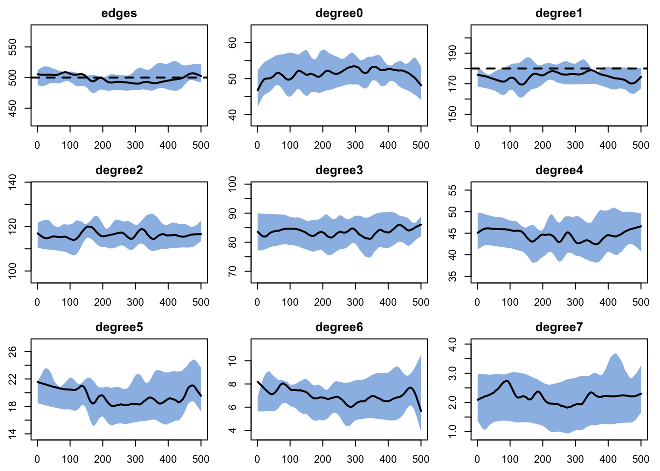

plot(dx)

42.4 Epidemic Model Parameterization

The epidemic model parameterization for any extension model consists of using the same three input functions as with built-in models.

First we start with the model parameters in param.net. Note that we have two new rates here: ei.rate and ir.rate. These control the transitions from E to I, and then I to R.

1param <- param.net(inf.prob = 0.5, act.rate = 2,
2                   ei.rate = 0.01, ir.rate = 0.01)

1

The two standard parameters, read inside infect by get_param(dat, "inf.prob") and get_param(dat, "act.rate").

2

The two new rates. These names are ones we chose; EpiModel does not know them and does not supply them. The same strings appear in the get_param() calls inside progress, and that correspondence is the only thing linking the parameter you set here to the value the module reads. A mismatch is not silent: get_param() stops with “There is no parameter called …”, so if you see that error, align the string here with the string in the module function.

Next we specify the initial conditions. Here we are specifying that there are 10 infectious individuals at the epidemic outset. If we wanted to initialize the model with persons only in the latent stage, we would need to set disease status as a nodal attribute on the network instead (following the same approach in the Serosorting Tutorial in Module 7).

init <- init.net(i.num = 10)

Finally, we specify the control settings in control.net. This is where an extension model differs most from a built-in one, so it is worth taking the arguments one at a time. The control.net Guide covers the full argument list.

1source("mod9-SEIR-fx.R")
2control <- control.net(type = NULL,
                       nsteps = 500,
                       nsims = 1,
                       ncores = 1,
3                       infection.FUN = infect,
4                       progress.FUN = progress,
5                       resimulate.network = FALSE)

1

Source the module functions first. control.net stores the function objects, captured as they exist at this moment, so infect and progress have to be defined before this call.

2

type is set to NULL in any extension model, because we are no longer asking EpiModel to pre-select which modules to run; the assembly is manual. This is not merely conventional: EpiModel stops with an error if type is non-NULL while any user module is present, and progress.FUN below is a user module.

3

infection.FUN is the slot for the infection process, and it defaults to NULL. On the built-in path EpiModel fills it from type; because we set type = NULL, nothing fills it, so supplying our own infect is required rather than optional. Without it the model would run no transmission at all.

4

progress.FUN adds a new module. control.net has no argument by that name, so it arrives through ... as a user module, and EpiModel runs every user module before every built-in module. progress therefore fires before infect at each time step, whatever order we write them in here. One visible consequence: a node exposed at step t cannot progress out of E until step t+1, because progress has already run by the time infect creates it. Replacing the built-in recovery module instead would not be equivalent, since recovery.FUN is a built-in slot and would run after infection. Use the module.order argument if you need to control this directly.

5

resimulate.network is set to FALSE explicitly. This is the default, so the line is not necessary, but it is a reminder that this is a model without network feedback.

In the R scripts that we include with this tutorial, you will see that we have two separate R script files (this rendered page shows the function definitions inline for reading, but it still sources them from the separate mod9-SEIR-fx.R, the same split as the downloadable scripts). One file contains the module functions, and the other contains all the other code to parameterize and run the model. We do this because it allows for easier interaction with the functions in browser mode. I will demonstrate this live next. But in general, placing the functions in a separate file conceptually disentangles the model functionality from the model parameterization. One practical consequence of the sourcing rule above: if you edit a module function, re-sourcing the file is not enough on its own, because control.net already captured the old version. Rebuild the control object as well.

42.5 Epidemic Simulation

Finally we are ready to do the epidemic model simulation and analysis. This is done using the same approach as the built-in models. We will start with running one model in the browser mode interactively.

sim <- netsim(est, param, init, control)

And then go back, comment out the browser lines, re-source the functions, and run a full-scale model with 10 simulations.

source("mod9-SEIR-fx.R")
control <- control.net(type = NULL,
                       nsteps = 500,
                       nsims = 10,
                       ncores = 5,
                       infection.FUN = infect,
                       progress.FUN = progress,
                       resimulate.network = FALSE)
sim <- netsim(est, param, init, control)

Once the model simulation is complete, we can work with the model object just like a built-in model. Start by printing the output to see what is available. Because this is an extension (type = NULL), the printout also includes the Model Functions section promised earlier, listing exactly the modules that ran, our infect and progress alongside the standard bookkeeping modules.

print(sim)

EpiModel Simulation
=======================
Model class: netsim

Simulation Summary
-----------------------
Model type:
No. simulations: 10
No. time steps: 500
No. NW groups: 1

Fixed Parameters
---------------------------
inf.prob = 0.5
act.rate = 2
ei.rate = 0.01
ir.rate = 0.01
groups = 1

Model Functions
-----------------------
initialize.FUN 
resim_nets.FUN 
summary_nets.FUN 
infection.FUN 
nwupdate.FUN 
prevalence.FUN 
verbose.FUN 
progress.FUN 

Model Output
-----------------------
Variables: s.num i.num num ei.flow ir.flow e.num r.num 
se.flow
Networks: sim1 ... sim10
Transmissions: sim1 ... sim10

Formation Statistics
----------------------- 
        Target Sim Mean Pct Diff Sim SE Z Score SD(Sim Means) SD(Statistic)
edges      500  501.438    0.288  1.772   0.811         8.133        21.394
degree1    180  174.926   -2.819  0.644  -7.885         3.639        11.601


Duration Statistics
----------------------- 
      Target Sim Mean Pct Diff Sim SE Z Score SD(Sim Means) SD(Statistic)
edges     25   24.987   -0.052  0.091  -0.142         0.308         1.059

Dissolution Statistics
----------------------- 
      Target Sim Mean Pct Diff Sim SE Z Score SD(Sim Means) SD(Statistic)
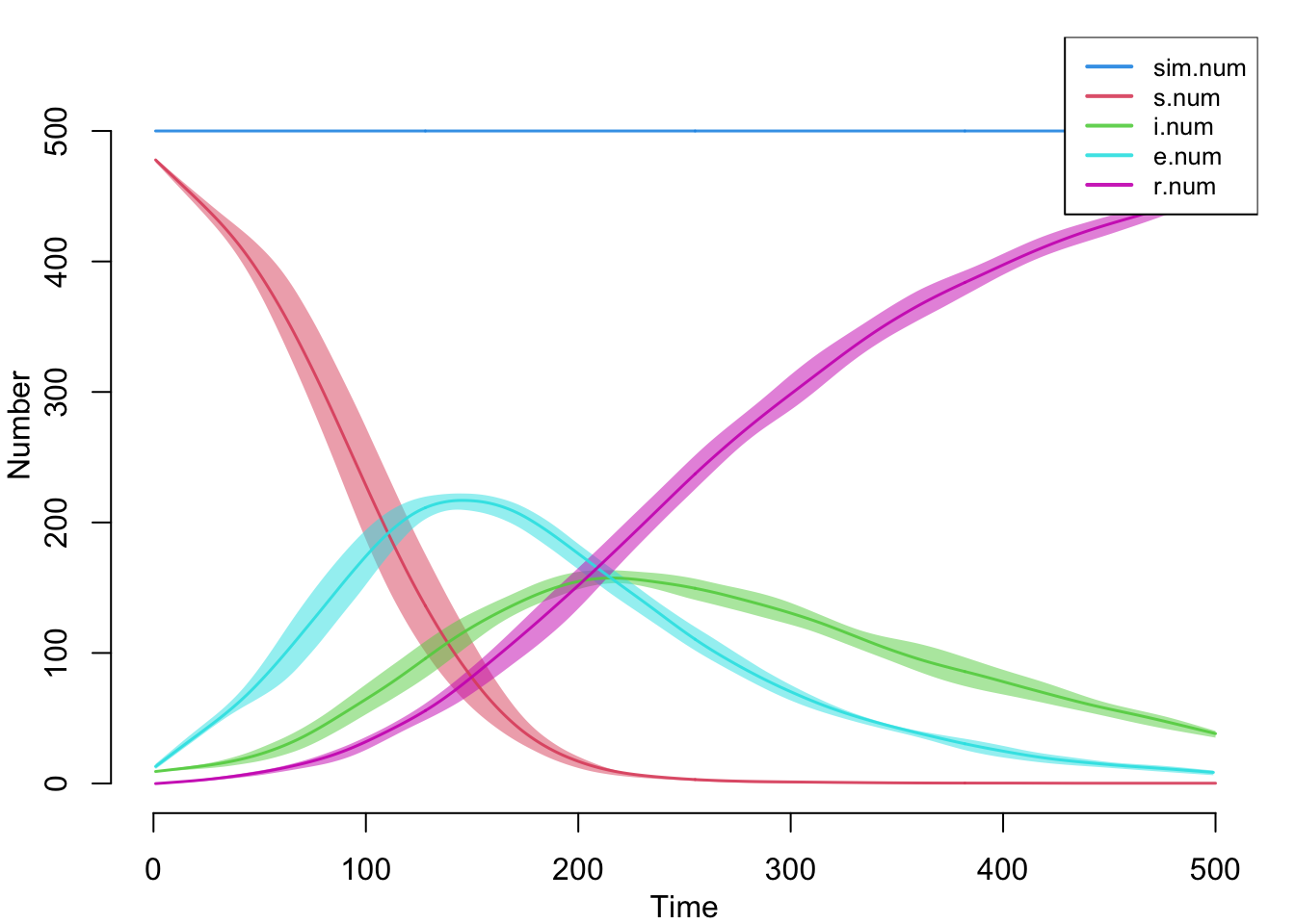
edges   0.04     0.04    0.179      0    0.58             0         0.009

Here is the default plot with all the compartment sizes over time. This includes the new summary statistics we tracked in the disease progression function.

par(mar = c(3, 3, 1, 1), mgp = c(2, 1, 0))
plot(sim)

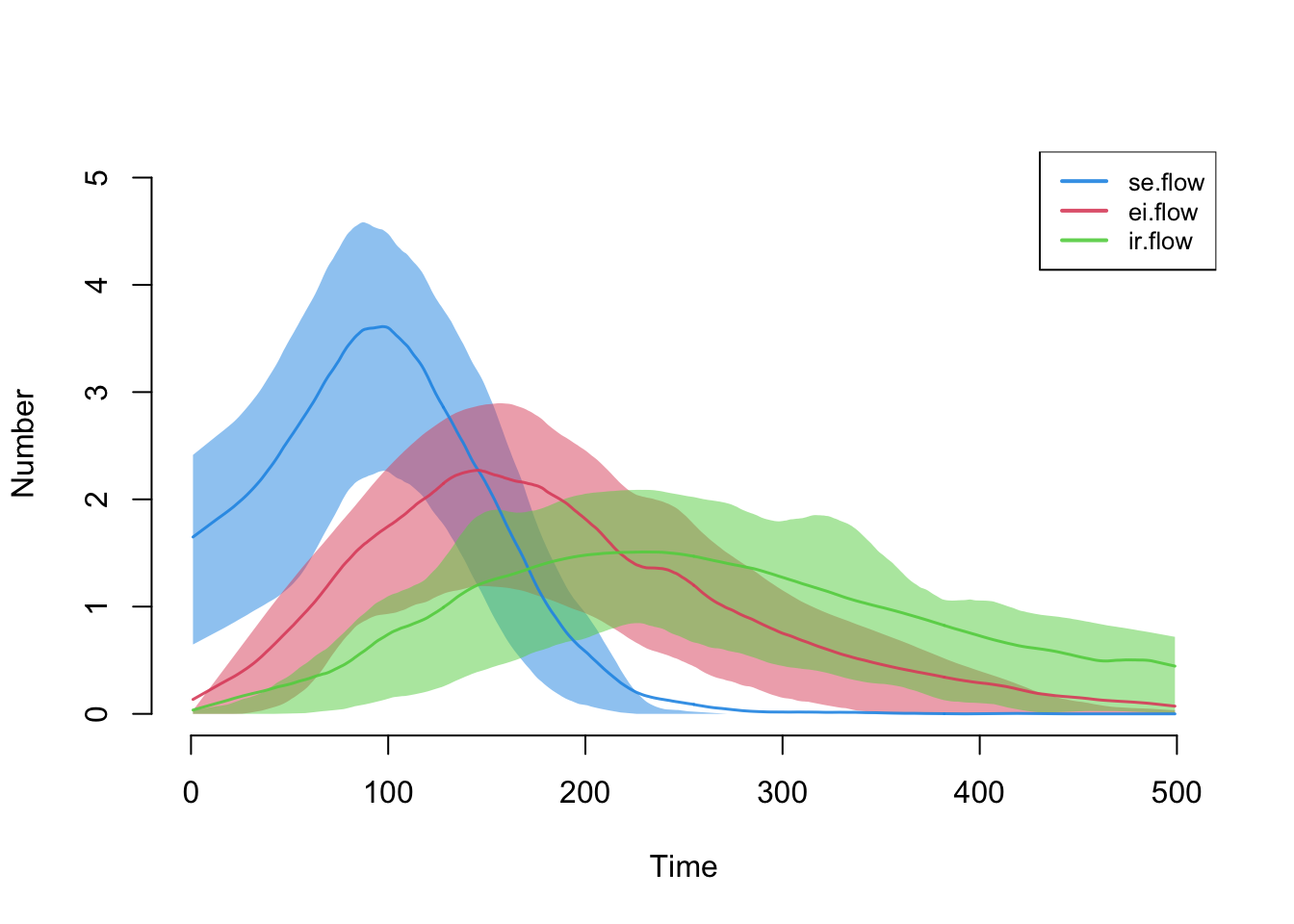
Here are the flow sizes, including the new se.flow incidence tracker that we established in the new infection function.

plot(sim, y = c("se.flow", "ei.flow", "ir.flow"), legend = TRUE)

Finally, here is the data frame output from the model, with rows limited to time step 100 across all 10 simulations.

df <- as.data.frame(sim)
df[which(df$time == 100), ]

     sim time s.num i.num num ei.flow ir.flow e.num r.num se.flow
100    1  100   182    76 500       5       0   206    33       3
600    2  100   186    76 500       1       1   200    36       2
1100   3  100   231    67 500       3       1   170    27       5
1600   4  100   185    81 500       4       0   197    31       6
2100   5  100   218    60 500       2       1   185    35       2
2600   6  100   214    76 500       2       0   176    29       5
3100   7  100   280    52 500       0       0   145    23       0
3600   8  100   202    88 500       2       0   182    24       4
4100   9  100   150    91 500       0       1   216    39       4
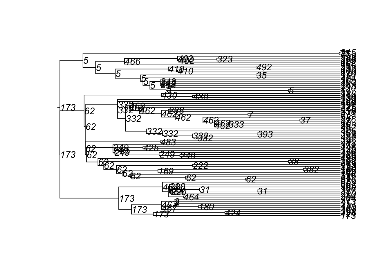
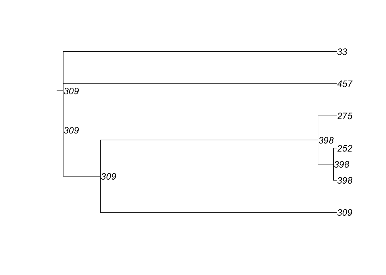
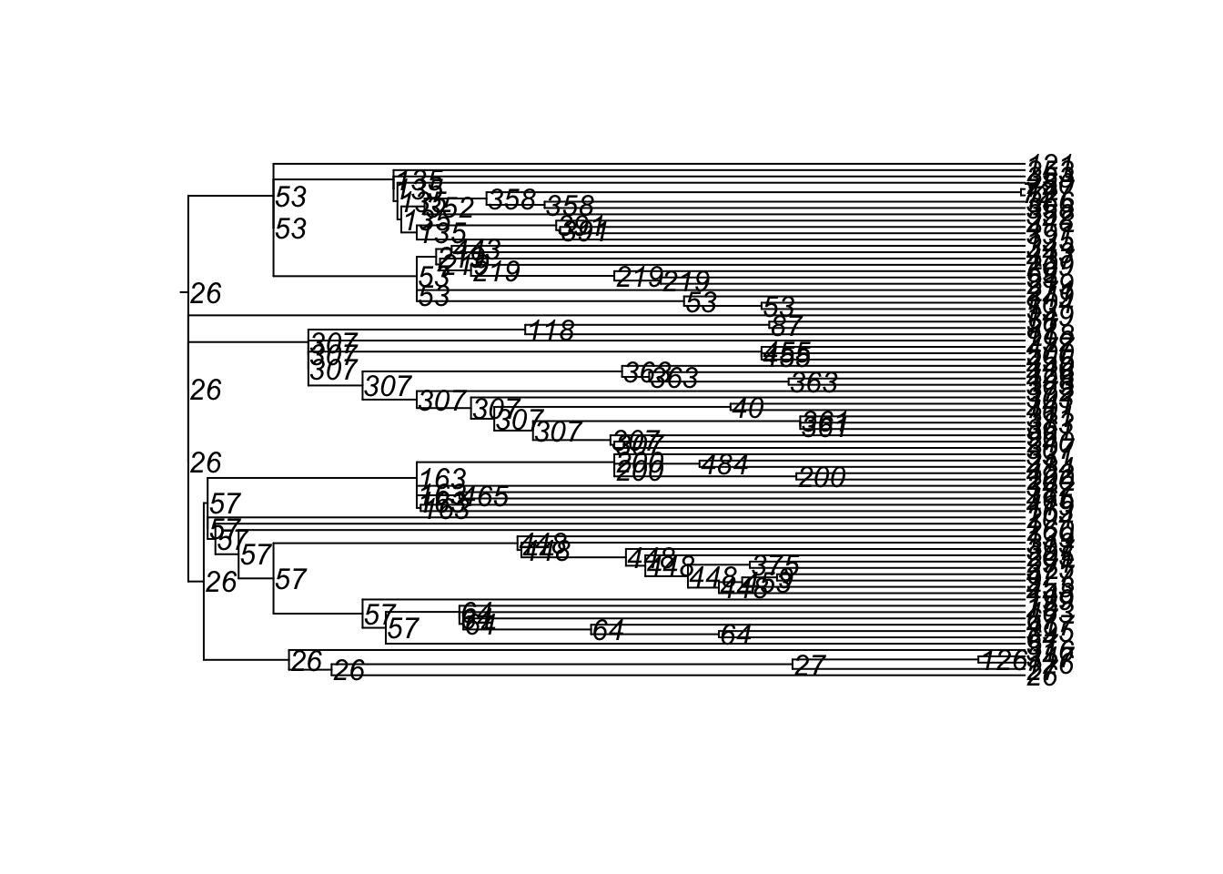
4600  10  100   233    61 500       3       0   170    28       8

The transmission matrix records, for each newly infected node, an attributed source (its infector). Below we plot a few of the transmission trees; each traces the onward infections from one initially infected node. A large epidemic descends from a handful of seeds into a few very large trees, so we show a few small-to-moderate ones rather than all of them, to keep the branching legible.

tm1 <- get_transmat(sim)

# get_transmat() returns at most one infector per newly infected node per step:
# if a susceptible had several infected partners transmit in the same step,
# EpiModel resolves that to a single attributed source (chosen at random by
# default, via the deduplicate argument). So "who infected whom" here is one
# plausible source per infection, not a claim that we observed the true one. In
# this SEIR model each node is infected only once, so tm1 is already a clean
# forest; we then plot only the three smallest trees that have at least three
# nodes, skipping the trivial one- and two-node ones, so the branching stays
# legible.
tmf <- tm1

tree_size <- function(root) {
  ids <- root
  repeat {
    kids <- tmf$sus[tmf$inf %in% ids]
    if (all(kids %in% ids)) break
    ids <- union(ids, kids)
  }
  length(ids)
}
roots <- setdiff(unique(tmf$inf), unique(tmf$sus))
sizes <- vapply(roots, tree_size, integer(1))
keep  <- head(roots[order(sizes)][sort(sizes) >= 3], 3)
if (length(keep) < 1) keep <- head(roots[order(sizes)], 3)

lineage <- keep
repeat {
  kids <- tmf$sus[tmf$inf %in% lineage]
  if (all(kids %in% lineage)) break
  lineage <- union(lineage, kids)
}
tm_sub <- tmf[tmf$inf %in% lineage, ]
class(tm_sub) <- class(tm1)

plot(tm_sub)

found multiple trees, returning a list of 3phylo objects