21 SIS Epidemic Across a Dynamic Network
We build and simulate a network-based epidemic model in EpiModel. EpiModel represents the contact network of an entire population, not a sample of it, and estimates it with a temporal exponential-family random graph model (TERGM). The TERGM lets us specify how edges form and dissolve as a function of individual-level, dyad-level, and network-level patterns: density, degree, assortativity, and others.
The process has two stages. First we estimate the temporal ERGM. Then we simulate a dynamic network from that fit, and simulate the epidemic on top of it.
In this tutorial, we work through a model of a Susceptible-Infected-Susceptible (SIS) epidemic. One example of an SIS disease would be a bacterial sexually transmitted infection such as Gonorrhea, in which individuals may acquire infection from sexual contact with an infected partner, and then recover from infection either through natural clearance or through antibiotic treatment.
Network modeling is not limited to STIs. The same formation and dissolution machinery applies to directly transmitted infections, such as a respiratory pathogen spreading over household, workplace, or school contact networks, where the edges represent the relevant person-to-person contacts rather than sexual partnerships.
Different model types excel at different questions. Some questions, or settings in which there is little behavioral data on who contacts whom, lend themselves to compartmental models; and as Module 5 shows, a discrete-time network model collapses to the dynamics a compartmental model produces once partnerships are redrawn every step. Sexually transmitted infections are a particularly natural fit for network models, because their contact networks are sparse and highly structured. Network models have also proven useful for respiratory infections, for both etiological and intervention questions, as the SARS-CoV-2 capstone in Module 13 demonstrates; such models tend to be more complex, since a respiratory contact network is denser and shifts faster than a sexual one.
We will use a simplifying assumption of a closed population, in which there are no entries or exits from the network; this may be justified by the short time span over which the epidemic will be simulated.
Download the R script to follow along with this tutorial here.
21.1 Network Model Estimation
To get started, load the EpiModel library.
The first step in our network model is to specify a network structure, including features like size and nodal attributes. The network_initialize function creates an object of class network. Below we show an example of initializing a network of 500 nodes, with no edges between them at the start. Edges represent sexual partnerships (mutual person-to-person contact), so this is an undirected network.
The sizes of the networks used in this course are smaller than what might be used for a research-level model; we do this to reduce computational waiting time during the examples. Larger network sizes over longer time intervals are typically used for research purposes.
21.1.1 Model Parameterization
This example will start simple, with a formula that represents the network density and the level of concurrency (overlapping sexual partnerships) in the population. This is a dyad-dependent ERGM, since the probability of edge formation between any two nodes depends on the existence of edges between those nodes and other nodes. The concurrent term is defined as the number of nodes with at least two partners at any time. Following the notation of the tergm package, we specify this using a right-hand side (RHS) formula. In addition to concurrency, we add a third formation term to cap the degree distribution. This term, degrange(from = 4), is given a target statistic of 0 (below), which drives the number of nodes with four or more partners to zero and so caps the momentary degree of any person at 3. It is a formation term like edges and concurrent, not the separate constraints= argument of netest introduced further below. A cap like this is a modeling assumption about the limits of concurrent partnering. Be careful not to justify it by pointing to a survey that top-codes partnerships (for example, one that asks respondents only about their 3 most recent partners): top-coding censors what we can observe about a person’s degree, but it does not establish that anyone’s true degree is capped at 3. That is a measurement limit, not a structural one.
Target statistics are the input mechanism for formation model terms. The order matters and nothing labels it: target.stats is a bare vector, and its elements are matched positionally to the terms in formation. This is the single most common source of confusion when getting started, so we write it out one term per line:
- 1
-
edges. A function of mean degree: \(edges = \text{mean degree} \times \frac{N}{2}\). At an arbitrarily specified mean degree of 0.7 on 500 nodes, that is \(0.7 \times 500 / 2 = 175\). - 2
-
concurrent. The number of nodes with two or more partners, so \(0.22 \times 500 = 110\). Note this is a count, not the proportion 0.22 we reasoned with. - 3
-
degrange(from = 4). The number of nodes with four or more partners, set to 0 to impose the cap.
An edges-only model implies an approximately Poisson degree distribution, so at a mean degree of 0.7 the probability of two or more partners is 1 - dpois(0, 0.7) - dpois(1, 0.7), about 16%. The assumed 22% is therefore roughly 40% more concurrency than chance alone would produce at this mean degree. Because we are holding mean degree fixed, the model can only buy that extra concurrency by moving people out of degree 1 and into degrees 0 and 2+, which you can see in the degree distribution in the diagnostics below.
The dissolution model is parameterized from a mean partnership duration estimated from cross-sectional egocentric data. It differs from the formation model in two respects.
First, the dissolution model is not estimated in the ERGM. It is instead passed in as a fixed coefficient, conditional on which the formation model is estimated. The dissolution model terms are calculated analytically using the dissolution_coefs function, the output of which is passed into the netest model estimation function.
Second, whereas formation models may be arbitrarily complex, dissolution models are limited to a set of dyad-independent terms. Dyad-independent means that a partnership’s probability of dissolution does not depend on the other partnerships in the network. These supported models are listed in the dissolution_coefs function help page.
The model we will use is an edges-only model, implying a homogeneous probability of dissolution for all partnerships in the network. The average duration of these partnerships will be specified at 50 time steps, which will be days in our model.
The unit of a time step is typically set by the key empirical dynamics in the model: demographic, partnership, and pathogen-related. Here there are no such empirical constraints, so we arbitrarily set the step to a day; other Module 4 tutorials use weeks.
Dissolution Coefficients
=======================
Dissolution Model: ~offset(edges)
Target Statistics: 50
Crude Coefficient: 3.89182
Mortality/Exit Rate: 0
Adjusted Coefficient: 3.89182
The output from this function indicates both an adjusted and crude coefficient. They are equivalent here because the adjustment applies only in an open population with entries and exits, where the coefficient must also account for partnerships that end when a partner leaves the population (through death or departure) rather than through dissolution itself. Upcoming workshop material will showcase when they differ as a result of exits from the network.
21.1.2 Model Estimation and Diagnostics
In EpiModel, network model estimation is performed with the netest function, which is a wrapper around the estimation functions in the ergm and tergm packages. The function arguments are as follows:
function (nw, formation, target.stats, coef.diss, constraints = NULL,
    coef.form = NULL, edapprox = TRUE, set.control.ergm = control.ergm(),
    set.control.tergm = control.tergm(MCMC.maxchanges = .Machine$integer.max),
    set.control.ergm.ego = NULL, verbose = FALSE, nested.edapprox = TRUE,
    ...)
NULL
The four arguments that must be specified with each function call are:
nw: an initialized empty network.formation: an RHS formation formula.target.stats: target statistics for the formation model.coef.diss: output object fromdissolution_coefs, containing the dissolution coefficients.
Other arguments that may be helpful to understand when getting started are:
constraints: this is another way of inputting model constraints (seehelp("ergm")).coef.form: sets the coefficient values of any offset terms in the formation model (those that are not explicitly estimated but fixed).edapprox: selects the dynamic estimation method. IfTRUE(the default), uses the approximation method; ifFALSE, the direct method.- Direct method: uses the functionality of the
tergmpackage to estimate the separable formation and dissolution models for the network. This is often not used because of computational time. - Approximation method: uses
ergmestimation for a cross-sectional network (the prevalence of edges) with an analytic adjustment of the edges coefficient to account for dissolution (i.e., transformation from prevalence to incidence). This approximation method may introduce bias into estimation in certain cases (high density and short durations) but these are typically not a concern for the low density cases in epidemiologically relevant networks.
- Direct method: uses the functionality of the
21.1.2.1 Estimation
Because we have a dyad-dependent model, MCMC will be used to estimate the coefficients of the model given the target statistics. We leave edapprox at its default, so this fit uses the edges dissolution approximation (edapprox = TRUE), which is the method the diagnostics below assess.
21.1.2.2 Diagnostics
There are two forms of model diagnostics for a dynamic ERGM fit with netest: static and dynamic diagnostics. When the approximation method has been used, static diagnostics check the fit of the cross-sectional model to target statistics. Dynamic diagnostics check the fit of the model adjusted to account for edge dissolution.
When running a dynamic network simulation, it is good to start with the dynamic diagnostics, and if there are fit problems, work back to the static diagnostics to determine if the problem is due to the cross-sectional fit itself or with the dynamic adjustment (i.e., the approximation method). A proper fitting ERGM using the approximation method does not guarantee well-performing dynamic simulations.
Here we will examine dynamic diagnostics only. These are run with the netdx function, which simulates from the model fit object returned by netest. One must specify the number of simulations from the dynamic model and the number of time steps per simulation. Choice of both simulation parameters depends on the stochasticity in the model, which is a function of network size, model complexity, and other factors. The nwstats.formula contains the network statistics to monitor in the diagnostics: it may contain statistics in the formation model and also others. By default, it is the formation model. Finally, we are keeping the “timed edgelist” (a record of every partnership with its start and end time) with keep.tedgelist.
We have also built parallelization into the EpiModel simulation functions, so it is also possible to run multiple simulations at the same time using your computer’s multi-core design. You can find the number of cores in your system with:
Then you can run the multi-core simulations by specifying ncores, as in the diagnostics below.
Throughout these tutorials we set ncores = 5, which runs the stochastic replicates on up to five CPU cores in parallel. Most laptops have at least this many, and the parallel runs are noticeably faster. You do not need to change this even if your machine has fewer cores. EpiModel automatically caps ncores at the number of cores you actually have, so ncores = 5 runs correctly everywhere (on a single-core machine it simply runs serially, just more slowly). If you would rather set the value yourself, check your core count with parallel::detectCores() and pass that number, or set ncores = 1 to force fully serial execution.
Printing the object will show the object structure and diagnostics. Both formation and duration diagnostics show a good fit relative to their targets. For the formation diagnostics, the mean statistics are the mean of the cross sectional statistics at each time step across all simulations. The Pct Diff column shows the relative difference between the mean and targets. For a first read, judge the fit from the Sim Mean and Pct Diff columns together with the plots below; the remaining columns (Sim SE, Z Score, and the two SD columns) report Monte Carlo error and between- versus within-simulation variability, and can be set aside for now. There are two forms of dissolution diagnostics. The edge duration row shows the mean duration of partnerships across the simulations; calculating this involves some imputation due to the length censoring at the start of the simulation. The next row shows the percent of current edges dissolving at each time step; this can be less intuitive than duration, but it does not require the imputation. The two are reciprocals of each other: if the mean duration is 50 days, we expect 1/50 of edges (2%) to dissolve each day.
EpiModel Network Diagnostics
=======================
Diagnostic Method: Dynamic
Simulations: 10
Time Steps per Sim: 1000
Formation Diagnostics
-----------------------
Target Sim Mean Pct Diff Sim SE Z Score SD(Sim Means) SD(Statistic)
edges 175 174.903 -0.056 1.079 -0.09 1.845 12.381
meandeg NA 0.700 NA 0.004 NA 0.007 0.050
degree0 NA 272.555 NA 1.291 NA 2.164 13.402
degree1 NA 118.428 NA 0.519 NA 1.221 9.642
degree2 NA 95.675 NA 0.603 NA 1.592 10.162
degree3 NA 13.342 NA 0.210 NA 0.720 3.840
degree4 NA 0.000 NA NaN NA 0.000 0.000
concurrent 110 109.018 -0.893 0.728 -1.35 1.537 11.326
Duration Diagnostics
-----------------------
Target Sim Mean Pct Diff Sim SE Z Score SD(Sim Means) SD(Statistic)
edges 50 50.94 1.88 0.288 3.265 0.812 3.489
Dissolution Diagnostics
-----------------------
Target Sim Mean Pct Diff Sim SE Z Score SD(Sim Means) SD(Statistic)
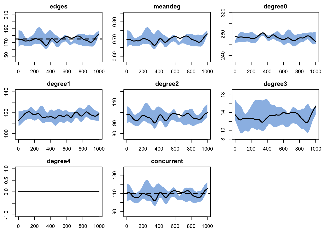
edges 0.02 0.02 -1.172 0 -2.211 0 0.011Plotting the diagnostics object will show the time series of the target statistics against any targets. By default, the mean lines are smoothed and drawn with a thicker line width, and each statistic is plotted in a separate panel. The black dashed lines show the value of the target statistics for any terms in the model. Similar to the numeric summaries, the plots show a good fit over the time series.
The simulated network statistics from diagnostic object may be extracted into a data.frame with get_nwstats.
time sim edges meandeg degree0 degree1 degree2 degree3 degree4 concurrent
1 1 1 176 0.704 268 124 96 12 0 108
2 2 1 177 0.708 269 121 97 13 0 110
3 3 1 177 0.708 269 121 97 13 0 110
4 4 1 179 0.716 269 116 103 12 0 115
5 5 1 180 0.720 267 118 103 12 0 115
6 6 1 183 0.732 265 117 105 13 0 118
7 7 1 185 0.740 264 116 106 14 0 120
8 8 1 185 0.740 267 112 105 16 0 121
9 9 1 183 0.732 267 116 101 16 0 117
10 10 1 181 0.724 268 119 96 17 0 113
11 11 1 182 0.728 268 118 96 18 0 114
12 12 1 186 0.744 269 112 97 22 0 119
13 13 1 181 0.724 272 112 98 18 0 116
14 14 1 181 0.724 271 112 101 16 0 117
15 15 1 179 0.716 274 107 106 13 0 119
16 16 1 178 0.712 274 108 106 12 0 118
17 17 1 177 0.708 272 113 104 11 0 115
18 18 1 174 0.696 273 117 99 11 0 110
19 19 1 174 0.696 274 116 98 12 0 110
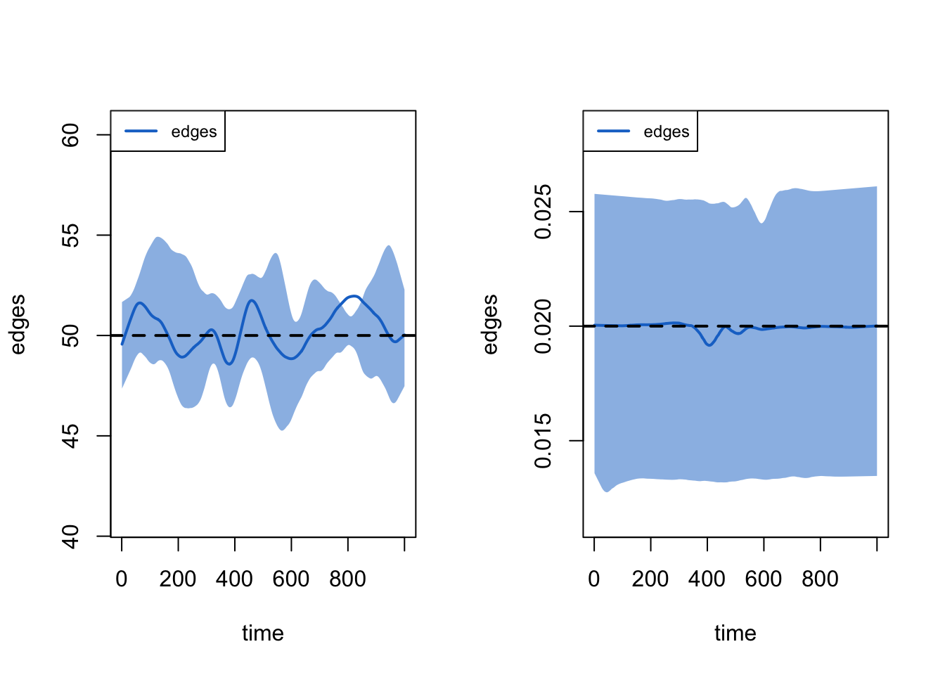
20 20 1 171 0.684 276 116 98 10 0 108The dissolution model fit may also be assessed with plots by specifying either the duration or dissolution type, as defined above. The duration diagnostic is based on the average age of edges at each time step, up to that time step. An imputation algorithm is used for left-censored edges (i.e., those that exist at t1); you can turn off this imputation to see the effects of censoring with duration.imputed = FALSE. Both metrics show a good fit of the dissolution model to the target duration of 50 time steps.
The timed edgelist records every partnership with its onset and terminus. Edges that already exist at the first time step are recorded with an onset of 0, the start of the observation window, and onset.censored is FALSE because that recorded spell begins exactly at the window’s edge. Their true start is earlier and unknown, and that is the left-censoring the duration diagnostic above imputes for when it estimates edge ages. The as.data.frame function extracts the edgelist object.
   onset terminus tail head onset.censored terminus.censored duration edge.id
1      0       59    1   54          FALSE             FALSE       59       1
2      0       69    1  143          FALSE             FALSE       69       2
3      0       57    4  253          FALSE             FALSE       57       3
4      0       14    4  495          FALSE             FALSE       14       4
5      0       19    5  320          FALSE             FALSE       19       5
6      0       48    8   43          FALSE             FALSE       48       6
7      0       88   11   56          FALSE             FALSE       88       7
8      0       95   13  188          FALSE             FALSE       95       8
9      0       28   15  424          FALSE             FALSE       28       9
10     0       58   19   54          FALSE             FALSE       58      10
11     0       34   19  460          FALSE             FALSE       34      11
12     0       79   24  406          FALSE             FALSE       79      12
13     0       15   28  130          FALSE             FALSE       15      13
14     0       12   28  240          FALSE             FALSE       12      14
15     0        8   33  229          FALSE             FALSE        8      15
16     0        6   33  478          FALSE             FALSE        6      16
17     0       16   34   95          FALSE             FALSE       16      17
18   268      290   34   95          FALSE             FALSE       22      17
19     0       84   34  464          FALSE             FALSE       84      18
20     0       34   35  471          FALSE             FALSE       34      19
If the model diagnostics had suggested a poor fit, then additional diagnostics and fitting would be necessary, especially the cross-sectional diagnostics (setting dynamic to FALSE in netdx). Note that the number of simulations may be very large here and there are no time steps specified because each simulation is a cross-sectional network.
The plots now represent individual simulations from an MCMC chain, rather than time steps.
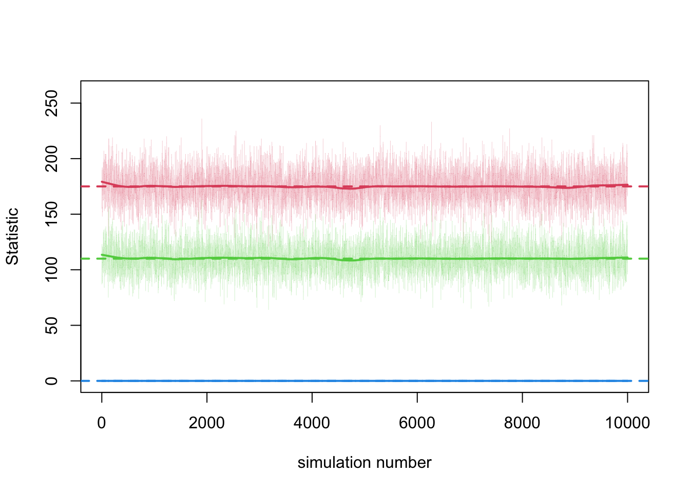
This lack of temporality is now evident when looking at the raw data.
   sim edges concurrent deg4+
1    1   170        106     0
2    2   183        114     0
3    3   197        126     0
4    4   155         93     0
5    5   166        100     0
6    6   195        116     0
7    7   179        111     0
8    8   202        133     0
9    9   178        114     0
10  10   169        102     0
11  11   174        102     0
12  12   156        101     0
13  13   163        104     0
14  14   166         99     0
15  15   170        100     0
16  16   159        103     0
17  17   136         81     0
18  18   171        108     0
19  19   166        104     0
20  20   168        105     0
If the cross-sectional model fits well but the dynamic model does not, then the direct estimation method described above may be necessary, setting edapprox = FALSE to fit the separable formation and dissolution models directly rather than using the edges dissolution approximation. If the cross-sectional model does not fit well, different control parameters for the ERGM estimation may be necessary (see the help file for netdx for instructions).
21.2 Epidemic Simulation
EpiModel simulates disease epidemics over dynamic networks by integrating dynamic model simulations with the simulation of other epidemiological processes such as disease transmission and recovery. Like the network model simulations, these processes are also simulated stochastically so that the range of potential outcomes under the model specifications is estimated.
The specification of epidemiological processes to model may be arbitrarily complex, but EpiModel includes a number of “built-in” model types within the software. Beyond these, custom processes can be written as R functions and plugged into the simulation at defined points. That is the subject of NME-II, which picks up exactly here. For now we start simple, with an SIS epidemic built entirely from the built-in functionality.
21.2.1 Epidemic Model Parameters
Our SIS model will rely on three parameters. The act rate is the number of sexual acts that occur within a partnership per time step. The overall frequency of acts per person per time step is a function of the number of ongoing partnerships (mean degree) and this act rate parameter. The infection probability is the risk of transmission given contact with an infected person. The recovery rate for an SIS epidemic is the speed at which infected individuals become susceptible again. For a bacterial STI like gonorrhea, this may be a function of biological attributes like sex or use of therapeutic agents like antibiotics.
If you have built a compartmental model, you wrote the infection flow as \(\beta S I / N\), and you built \(\beta\) out of two pieces: a per-contact transmission probability, and a contact rate.
EpiModel splits that same idea across three places, and the split is the whole point of the module.
inf.probis the per-act transmission probability. It is the same quantity you already know.act.rateis the number of acts per partnership per time step.- The number of partners is not a parameter at all. It is the network.
In a compartmental model the contact rate is a number you choose, and it is the same for everyone. Here it is an outcome of the network: who has how many partners, who those partners are, and how long the partnerships last. That is why we spent Modules 1 through 3 building a statistical model for the network before writing down a single epidemic parameter.
EpiModel uses three helper functions to input epidemic parameters, initial conditions, and other control settings for the epidemic model. Each function holds a distinct part of the specification: param.net holds the epidemic-process parameters (transmission probability, act rate, recovery rate), init.net holds the initial conditions (how many people start infected), and control.net holds the simulation settings and engine (model type, number of simulations, number of time steps, and any added modules). First, we use the param.net function to input the per-act transmission probability in inf.prob and the number of acts per partnership per unit time in act.rate. The recovery rate implies that the average duration of disease is 10 days (1/rec.rate).
For initial conditions in this model, we only need to specify the number of infected individuals at the outset of the epidemic. The remaining individuals in the network will be classified as disease susceptible.
The control settings specify the structural elements of the model, and this is the function to understand well: control.net decides what the model is, where param.net only decides what its numbers are.
type is the most consequential argument. It selects which built-in modules EpiModel runs, and therefore what else you are required to supply: "SI" needs only inf.prob and act.rate; "SIS" adds rec.rate; "SIR" adds rec.rate and requires r.num in init.net for the recovered compartment. Setting type is how you choose the disease’s natural history.
nsims is the number of stochastic replicates. Run enough of them to characterize the run-to-run variability in outcomes; small or noisy models need more. nsteps is the number of time steps, set long enough to cover the time horizon of interest, here for the SIS epidemic to reach its endemic equilibrium. ncores runs the replicates in parallel across your machine’s cores.
Later modules add arguments to control.net for custom modules and other simulation machinery. For now, type, nsims, nsteps and ncores are the whole story.
21.2.2 Simulating the Epidemic Model
Once the model has been parameterized, simulating the model is straightforward. One must pass the fitted network model object from netest along with the parameters, initial conditions, and control settings to the netsim function. With a no-feedback model like this (i.e., there are no vital dynamics parameters), the full dynamic network time series is simulated at the start of each epidemic simulation, and then the epidemiological processes are simulated over that structure.
Printing the model output lists the inputs and outputs of the model. The output includes the sizes of the compartments (s.num is the number susceptible and i.num is the number infected) and flows (si.flow is the number of infections and is.flow is the number of recoveries). Methods for extracting this output are discussed below.
EpiModel Simulation
=======================
Model class: netsim

Simulation Summary
-----------------------
Model type: SIS
No. simulations: 5
No. time steps: 500
No. NW groups: 1

Fixed Parameters
---------------------------
inf.prob = 0.4
act.rate = 2
rec.rate = 0.1
groups = 1

Model Output
-----------------------
Variables: s.num i.num num si.flow is.flow
Networks: sim1 ... sim5
Transmissions: sim1 ... sim5

Formation Statistics
-----------------------
           Target Sim Mean Pct Diff Sim SE Z Score SD(Sim Means) SD(Statistic)
edges         175  172.583   -1.381  2.527  -0.956         5.441        14.210
concurrent    110  107.441   -2.326  1.630  -1.569         4.485        12.621
deg4+           0    0.000      NaN    NaN     NaN         0.000         0.000


Duration Statistics
-----------------------
      Target Sim Mean Pct Diff Sim SE Z Score SD(Sim Means) SD(Statistic)
edges     50   51.195    2.391  0.667   1.792         2.819         4.323

Dissolution Statistics
-----------------------
      Target Sim Mean Pct Diff Sim SE Z Score SD(Sim Means) SD(Statistic)
edges   0.02     0.02   -1.099      0  -1.048         0.001         0.011
21.2.3 Model Analysis
Now that the model has been simulated, the next step is to analyze the data. This includes plotting the epidemiological output, the networks over time, and extracting other raw data.
21.2.3.1 Epidemic Plots
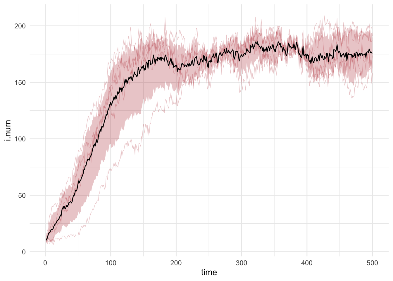
Plotting the output from the epidemic model using the default arguments will display the size of the compartments in the model across simulations. The means across simulations at each time step are plotted with lines, and the polygon band shows the inter-quartile range across simulations.
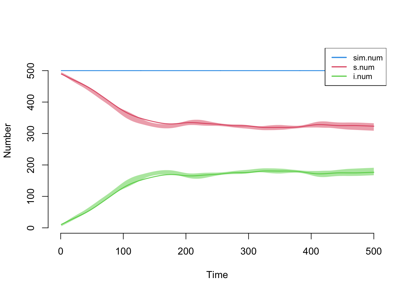
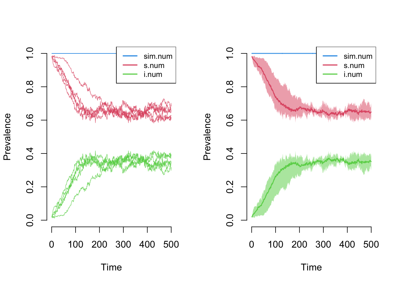
Graphical elements may be toggled on and off. The popfrac argument specifies whether to use the absolute size of compartments versus proportions.
Code
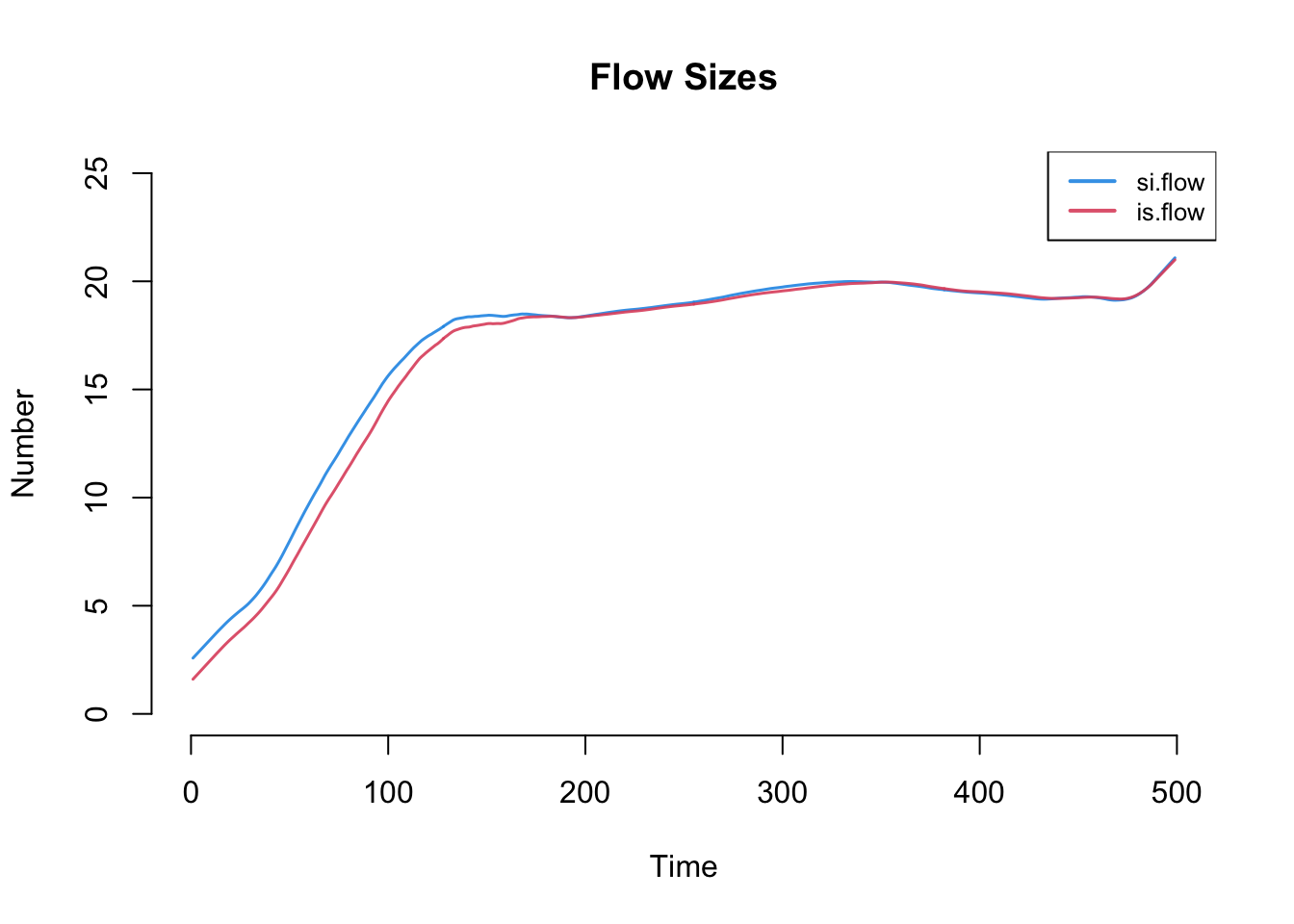
Whereas the default will print the compartment sizes, other elements of the simulation may be plotted by name with the y argument. Here we plot both flow sizes using smoothed means, which converge at model equilibrium by the end of the time series.
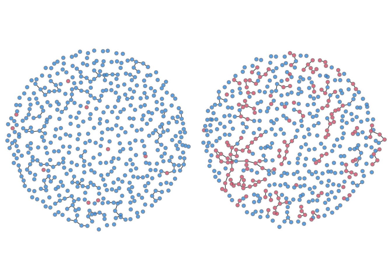
21.2.3.2 Network Plots
Another available plot type is a network plot to visualize the individual nodes and edges at a specific time point. Network plots are output by setting the type parameter to "network". To plot the disease infection status on the nodes, use the col.status argument: blue indicates susceptible and red infected. It is necessary to specify both a time step and a simulation number to plot these networks.
21.2.3.3 Time-Specific Model Summaries
The summary function with the output of netsim will show the model statistics at a specific time step. Here we output the statistics at the final time step, where the epidemic has reached its endemic equilibrium: a bit over a third of the population is infected and the rest remain susceptible. At equilibrium the S to I and I to S flows have come into balance, so prevalence stops changing even though infections and recoveries continue.
EpiModel Summary
=======================
Model class: netsim

Simulation Details
-----------------------
Model type: SIS
No. simulations: 5
No. time steps: 500
No. NW groups: 1

Model Statistics
------------------------------
Time: 500
------------------------------
           mean     sd    pct
Suscept.  313.8  6.380  0.628
Infect.   186.2  6.380  0.372
Total     500.0  0.000  1.000
S -> I     21.6  3.912     NA
I -> S     18.0  9.566     NA
------------------------------
21.2.3.4 Data Extraction
The as.data.frame function may be used to extract the model output into a data frame object for easy analysis outside of the built-in EpiModel functions. The function default will output the raw data for all simulations for each time step.
   sim time s.num i.num num si.flow is.flow
1    1    1   490    10 500      NA      NA
2    1    2   484    16 500       8       2
3    1    3   483    17 500       5       4
4    1    4   480    20 500       5       2
5    1    5   476    24 500       6       2
6    1    6   473    27 500       9       6
7    1    7   470    30 500       8       5
8    1    8   465    35 500       8       3
9    1    9   463    37 500       8       6
10 1 10 460 40 500 5 2 sim time s.num i.num num si.flow is.flow
2491 5 491 334 166 500 24 18
2492 5 492 337 163 500 15 18
2493 5 493 337 163 500 21 21
2494 5 494 330 170 500 27 20
2495 5 495 327 173 500 17 14
2496 5 496 334 166 500 12 19
2497 5 497 342 158 500 19 27
2498 5 498 340 160 500 22 20
2499 5 499 334 166 500 32 26
2500 5 500 321 179 500 20 7Notice that the output above shows all compartment and flow sizes as integers, reinforcing this as an individual-level model.
The out argument may be changed to specify the output of means across the models (with out = "mean").
   time s.num i.num num si.flow is.flow
1     1 490.0  10.0 500     NaN     NaN
2     2 485.0  15.0 500     6.0     1.0
3     3 482.2  17.8 500     4.6     1.8
4     4 479.2  20.8 500     5.6     2.6
5     5 475.8  24.2 500     6.0     2.6
6     6 472.8  27.2 500     6.0     3.0
7     7 468.8  31.2 500     5.6     1.6
8     8 467.6  32.4 500     4.6     3.4
9     9 466.4  33.6 500     5.0     3.8
10 10 465.4 34.6 500 5.6 4.6 time s.num i.num num si.flow is.flow
491 491 318.2 181.8 500 22.8 21.6
492 492 317.2 182.8 500 20.6 19.6
493 493 314.0 186.0 500 23.2 20.0
494 494 314.0 186.0 500 20.6 20.6
495 495 310.4 189.6 500 18.8 15.2
496 496 310.6 189.4 500 16.6 16.8
497 497 313.8 186.2 500 17.0 20.2
498 498 316.8 183.2 500 18.4 21.4
499 499 317.4 182.6 500 23.4 24.0
500 500 313.8 186.2 500 21.6 18.0The networkDynamic objects are stored in the netsim object, and may be extracted with the get_network function. By default the dynamic networks are saved, and contain the full edge history for every node that has existed in the network, along with the disease status history of those nodes.
NetworkDynamic properties:
  distinct change times: 502
  maximal time range: 0 until  Inf

 Dynamic (TEA) attributes:
  Vertex TEAs:    testatus.active

Includes optional net.obs.period attribute:
 Network observation period info:
  Number of observation spells: 2
  Maximal time range observed: 0 until 501
  Temporal mode: discrete
  Time unit: step
  Suggested time increment: 1

 Network attributes:
  vertices = 500
  directed = FALSE
  hyper = FALSE
  loops = FALSE
  multiple = FALSE
  bipartite = FALSE
  net.obs.period: (not shown)
  vertex.pid = tergm_pid
  total edges= 1899
    missing edges= 0
    non-missing edges= 1899

 Vertex attribute names:
    active status tergm_pid testatus.active vertex.names

 Edge attribute names not shown
One thing you can do with that network dynamic object is to extract the timed edgelist of all ties that existed for that simulation.
   onset terminus tail head onset.censored terminus.censored duration edge.id
1      0       39    1  382          FALSE             FALSE       39       1
2      0       34    2  148          FALSE             FALSE       34       2
3      0       49    2  291          FALSE             FALSE       49       3
4      0       14    5   99          FALSE             FALSE       14       4
5      0       78    5  112          FALSE             FALSE       78       5
6      0        2    7  337          FALSE             FALSE        2       6
7      0       35    8  127          FALSE             FALSE       35       7
8      0       25    8  290          FALSE             FALSE       25       8
9      0       64   13  189          FALSE             FALSE       64       9
10     0        5   18  386          FALSE             FALSE        5      10
11     0       54   20  408          FALSE             FALSE       54      11
12     0       80   21  285          FALSE             FALSE       80      12
13     0       68   23  178          FALSE             FALSE       68      13
14     0       42   23  225          FALSE             FALSE       42      14
15     0       46   23  427          FALSE             FALSE       46      15
16     0      211   24   47          FALSE             FALSE      211      16
17     0       41   24  268          FALSE             FALSE       41      17
18     0       38   24  487          FALSE             FALSE       38      18
19     0       50   25   61          FALSE             FALSE       50      19
20     0       99   26  264          FALSE             FALSE       99      20
21     0      101   27  166          FALSE             FALSE      101      21
22     0       39   29   65          FALSE             FALSE       39      22
23     0        8   30  253          FALSE             FALSE        8      23
24     0       78   31  260          FALSE             FALSE       78      24
25 0 45 32 147 FALSE FALSE 45 25At each time step, EpiModel finds every active tie with one susceptible partner and one infectious partner. These are the discordant edges, and they are the only place transmission can happen. For each one, EpiModel does not simulate the act.rate acts one at a time. It collapses them into a single per-partnership transmission probability, \(1 - (1 - p)^{a}\) (where \(p\) is the per-act probability inf.prob and \(a\) is act.rate), and makes one Bernoulli draw against that probability to decide whether infection passes along the edge this step. That combined probability is exactly the chance that at least one of \(a\) independent acts transmits, and it is the finalProb reported in the transmission matrix below.
This is the unit a network epidemic model actually operates on. A tie between two susceptibles does nothing; a tie between two infecteds does nothing. Only the discordant ones matter, and which ties are discordant changes at every step as the epidemic and the network both move.
We can also use the get_transmat function to generate a record of some key details about each transmission event that occurred. Shown below are the first 10 transmission events for simulation number 1. The at column gives the time step at which the transmission occurred. The sus column shows the unique ID of the previously susceptible, newly infected node in the event, and inf the ID of the transmitting node. network is the network layer on which the contact occurred, always 1 here; it only becomes useful in the multi-layer models of NME-II. infDur is the duration of the transmitting node’s infection at the time of transmission, transProb the per-act transmission probability, actRate the act rate, and finalProb the resulting per-partnership transmission probability at that time step.
# A tibble: 10 × 8
# Groups:   at, sus [10]
      at   sus   inf network infDur transProb actRate finalProb
   <int> <int> <int>   <int>  <dbl>     <dbl>   <dbl>     <dbl>
 1     2    66   187       1      1       0.4       2      0.64
 2     2   119   343       1      6       0.4       2      0.64
 3     2   143   181       1      1       0.4       2      0.64
 4     2   199   442       1     21       0.4       2      0.64
 5     2   247   343       1      6       0.4       2      0.64
 6     2   260   378       1     33       0.4       2      0.64
 7     2   262   343       1      6       0.4       2      0.64
 8     2   365   378       1     33       0.4       2      0.64
 9     3   153    66       1      1       0.4       2      0.64
10     3   241   428       1      1       0.4       2      0.64
21.2.3.5 Data Exporting and Plotting with ggplot
We built in plotting methods directly for netsim class objects so you can easily plot multiple types of summary statistics from the simulated model object. However, if you prefer an external plotting tool in R, such as ggplot, it is easy to extract the data in tidy format for analysis and plotting. Here is an example of how to do so for our model above. See the help for the ggplot if you are unfamiliar with this syntax.
Code
df <- as.data.frame(sim)
df.mean <- as.data.frame(sim, out = "mean")

library(ggplot2)
ggplot() +
  geom_line(data = df, mapping = aes(time, i.num, group = sim), alpha = 0.25,
            lwd = 0.25, color = "firebrick") +
  geom_bands(data = df, mapping = aes(time, i.num),
             lower = 0.1, upper = 0.9, fill = "firebrick") +
  geom_line(data = df.mean, mapping = aes(time, i.num)) +
  theme_minimal()