24  Working with Nodal Attributes in Network Models

Our examples so far were all built on a set of nodes that were homogeneous, except for infectious status. In this tutorial, we’ll introduce two groups that can systematically differ in their behavior and/or their epidemic parameters (e.g. average duration of infection). We’ll motivate our example with a heterosexual network in which the groups represent females and males in the population.

Note

Download the R script to follow along with this tutorial here.

24.1 Getting Started

To get started, load the EpiModel library.

library(EpiModel)

We also recommend that you clear your environment to avoid any leftover objects from the last tutorials or labs.

rm(list = ls())

And we will set the seed to ensure reproducible results:

set.seed(12345)

24.2 Network Model

For the network model parameterization, we’ll fit a two-group model with a differential degree distribution by group. We will do so using the special group attribute.

In core EpiModel, the group attribute has a special role for these built-in models that we are exploring in this course. It allows for easy parameterization of heterogeneous epidemic parameters (e.g., group-specific recovery rates). This functionality requires that group takes only two values, which must be 1 and 2. In our example, group 1 will represent women and group 2 men.

The group attribute makes life easier in this specific circumstance. In future examples, we can, and will, use other nodal attributes that can take more values (e.g. age or race) and model their impacts on network structure specifically. (Epidemic parameters can also be stratified by an arbitrary number of attributes with arbitrary values; however, this requires some additional programming of the epidemic modules in EpiModel. This is covered in the NME II workshop.)

24.2.1 Initialization

First we set up the network. The number of nodes in each group will be 250:

num.g1 <- num.g2 <- 250
n <- num.g1 + num.g2
nw <- network_initialize(n)
nw

 Network attributes:
  vertices = 500 
  directed = FALSE 
  hyper = FALSE 
  loops = FALSE 
  multiple = FALSE 
  bipartite = FALSE 
  total edges= 0 
    missing edges= 0 
    non-missing edges= 0 

 Vertex attribute names: 
    vertex.names 

No edge attributes

We next define our nodal attribute group, and then set it on the network. We can print out the network again to see that it has been added to the list of vertex attributes. Remember, to access the special functionality associated with the group attribute, its values must be 1 and 2 only.

group <- rep(1:2, times = c(num.g1, num.g2))
nw <- set_vertex_attribute(nw, attrname = "group", value = group)
nw

 Network attributes:
  vertices = 500 
  directed = FALSE 
  hyper = FALSE 
  loops = FALSE 
  multiple = FALSE 
  bipartite = FALSE 
  total edges= 0 
    missing edges= 0 
    non-missing edges= 0 

 Vertex attribute names: 
    group vertex.names 

No edge attributes

We can use get_vertex_attribute to extract the same attribute from the network object:

get_vertex_attribute(nw, "group")

  [1] 1 1 1 1 1 1 1 1 1 1 1 1 1 1 1 1 1 1 1 1 1 1 1 1 1 1 1 1 1 1 1 1 1 1 1 1 1
 [38] 1 1 1 1 1 1 1 1 1 1 1 1 1 1 1 1 1 1 1 1 1 1 1 1 1 1 1 1 1 1 1 1 1 1 1 1 1
 [75] 1 1 1 1 1 1 1 1 1 1 1 1 1 1 1 1 1 1 1 1 1 1 1 1 1 1 1 1 1 1 1 1 1 1 1 1 1
[112] 1 1 1 1 1 1 1 1 1 1 1 1 1 1 1 1 1 1 1 1 1 1 1 1 1 1 1 1 1 1 1 1 1 1 1 1 1
[149] 1 1 1 1 1 1 1 1 1 1 1 1 1 1 1 1 1 1 1 1 1 1 1 1 1 1 1 1 1 1 1 1 1 1 1 1 1
[186] 1 1 1 1 1 1 1 1 1 1 1 1 1 1 1 1 1 1 1 1 1 1 1 1 1 1 1 1 1 1 1 1 1 1 1 1 1
[223] 1 1 1 1 1 1 1 1 1 1 1 1 1 1 1 1 1 1 1 1 1 1 1 1 1 1 1 1 2 2 2 2 2 2 2 2 2
[260] 2 2 2 2 2 2 2 2 2 2 2 2 2 2 2 2 2 2 2 2 2 2 2 2 2 2 2 2 2 2 2 2 2 2 2 2 2
[297] 2 2 2 2 2 2 2 2 2 2 2 2 2 2 2 2 2 2 2 2 2 2 2 2 2 2 2 2 2 2 2 2 2 2 2 2 2
[334] 2 2 2 2 2 2 2 2 2 2 2 2 2 2 2 2 2 2 2 2 2 2 2 2 2 2 2 2 2 2 2 2 2 2 2 2 2
[371] 2 2 2 2 2 2 2 2 2 2 2 2 2 2 2 2 2 2 2 2 2 2 2 2 2 2 2 2 2 2 2 2 2 2 2 2 2
[408] 2 2 2 2 2 2 2 2 2 2 2 2 2 2 2 2 2 2 2 2 2 2 2 2 2 2 2 2 2 2 2 2 2 2 2 2 2
[445] 2 2 2 2 2 2 2 2 2 2 2 2 2 2 2 2 2 2 2 2 2 2 2 2 2 2 2 2 2 2 2 2 2 2 2 2 2
[482] 2 2 2 2 2 2 2 2 2 2 2 2 2 2 2 2 2 2 2

24.2.2 Model specification

We are going to specify:

1. a constraint that all ties must be cross-sex
2. the expected total number of ties
3. the expected proportion of each sex that has concurrent ties at any point in time.

To do so, we begin by thinking through some basic logic to identify the rules that our model and its target statistics must obey.

First off, the total number of ties that females have with males must logically equal the total number of ties that males have with females. This logical rule is always the case when considering undirected ties between two groups.

The constraint above about all ties being cross-sex means that this logical relationship can be extended here to say that for this network, total number of ties for females must equal the the total number of ties for males. Note that this is not universally true, but only holds in this case because of the pure cross-sex tie constraint.

The total number of ties for a group equals the number of nodes in the group times the mean degree for that group. We specified above that the number of females and the number of males are equal. Therefore, we can further extend our logical rules to say that, for this network, the mean degree for females must equal the mean degree for males. Note again that this is not universally true, but only holds in this case because of both the pure cross-sex tie constraint and the fact that the two groups have the exact same population size.

We will thus set a single overall mean degree. We will chose a value of 0.66.

meandeg <- 0.66

Now we would like to consider the proportion of each group that has concurrent ties at any point in time. Is there a logical constraint on how these numbers relate to each other? Think about it before proceeding….

In general, there is no simple constraint here. For example, think of a population of 4 women and 4 men. Each woman has one partner, and for all four of them it’s man #1. The women have 0% concurrency while the men have 25%. What if the first two women are partners with man #1 and the other two with man #2? Now the men have 50% concurrency while the women still have 0%. There can be overall constraints on concurrency imposed by the mean degree (e.g. if it’s greater than 1 then someone has to have concurrent partners). And there are constraints at the extremes on the sex-specific values. But in general, they are pretty free to move independently.

So, we will specify the proportion of each sex that has concurrent partners: 5% for females, and 15% for males. It is common in empirical data to see the value higher for males than females.

pconc.g1 <- c(0.05)
pconc.g2 <- c(0.15)

As you progress into more complex network models, it is helpful to practice thinking through the logical relationships among your terms and their associated statistics carefully. This helps to ensure that you are including the right set of terms for your goal, and not over- or under-specifying the model. We dive into this more deeply in NME-II.

24.2.3 Formation model

Next, we specify the terms in our formation model. As usual, we want an edges term to model the overall mean degree.

The nodematch term is new: it allows one to model assortative or disassortative mixing across an attribute. We will use it to encode our assumption that all ties are cross-sex.

The concurrent term specifies the proportion of nodes expected to have concurrent partners at any point in time. It includes an option by argument, which takes the name of a nodal attribute on which the effect can be disaggregated. To tell it that we want to specify each group, we need to set the levels argument. There are multiple equivalent ways we could do this, including passing the specific values 1:2. However, using NULL is a more general way to say “all levels” without having to know the number of their values:

Putting this all together, we get:

formation <- ~edges + nodematch("group") + concurrent(by = "group", levels = NULL)

For the target statistics, we specify the number of edges as a function of mean degree. The target statistic for nodematch with a purely disassortative mixing model is 0: there are no edges between persons matched on the value of the group variable. Finally, we calculate the expected number of females and males with concurrent partners, respectively:

target.stats <- c(n*meandeg/2, 0, num.g1*pconc.g1, num.g2*pconc.g2)
target.stats

[1] 165.0   0.0  12.5  37.5

Note that it is perfectly fine for our target values for concurrent to not be whole numbers. How can that be, when the number of people with concurrent partners must be a whole number at any point in time? Because the average of a set of whole numbers (in our case, averaged over time) does not need to be a whole number.

24.2.4 Dissolution model

The dissolution model is parameterized the same as the prior example but with a shorter partnership duration than the first tutorial; we’ll go with 20 steps:

coef.diss <- dissolution_coefs(dissolution = ~offset(edges), duration = 20)
coef.diss

Dissolution Coefficients
=======================
Dissolution Model: ~offset(edges)
Target Statistics: 20
Crude Coefficient: 2.944439
Mortality/Exit Rate: 0
Adjusted Coefficient: 2.944439

24.2.5 Estimation

The netest function is used for network model fitting.

est <- netest(nw, formation, target.stats, coef.diss)

For the dynamic diagnostics, we simulate from the model fit. We’ll track not only the concurrent statistics but also the degree distribution as a whole:

dx <- netdx(est, nsims = 25, nsteps = 500, ncores = 5,
            nwstats.formula = ~edges + concurrent(by = "group") + degree(0:3, by = "group"))

Network Diagnostics
-----------------------
- Simulating 25 networks
- Calculating formation statistics

dx

EpiModel Network Diagnostics
=======================
Diagnostic Method: Dynamic
Simulations: 25
Time Steps per Sim: 500

Formation Diagnostics
----------------------- 
                  Target Sim Mean Pct Diff Sim SE Z Score SD(Sim Means)
edges              165.0  162.557   -1.481  0.494  -4.945         3.060
concurrent.group1   12.5   12.711    1.690  0.161   1.309         1.090
concurrent.group2   37.5   36.166   -3.556  0.181  -7.369         1.123
deg0.group.1          NA  106.825       NA  0.283      NA         1.829
deg1.group.1          NA  130.463       NA  0.269      NA         1.750
deg2.group.1          NA    7.934       NA  0.087      NA         0.634
deg3.group.1          NA    3.323       NA  0.055      NA         0.384
deg0.group.2          NA  131.863       NA  0.289      NA         1.969
deg1.group.2          NA   81.971       NA  0.240      NA         1.537
deg2.group.2          NA   29.112       NA  0.139      NA         0.988
deg3.group.2          NA    6.002       NA  0.067      NA         0.361
                  SD(Statistic)
edges                    11.113
concurrent.group1         3.581
concurrent.group2         5.092
deg0.group.1              8.031
deg1.group.1              7.987
deg2.group.1              2.838
deg3.group.1              1.835
deg0.group.2              7.122
deg1.group.2              7.233
deg2.group.2              4.785
deg3.group.2              2.349

Duration Diagnostics
----------------------- 
      Target Sim Mean Pct Diff Sim SE Z Score SD(Sim Means) SD(Statistic)
edges     20   20.005    0.027  0.078   0.068         0.369         1.528

Dissolution Diagnostics
----------------------- 
      Target Sim Mean Pct Diff Sim SE Z Score SD(Sim Means) SD(Statistic)
edges   0.05     0.05    0.066      0   0.219         0.001         0.017

The edges seem to have a small bias, due to the relatively short duration. This is confirmed when we plot the diagnostics:

plot(dx)

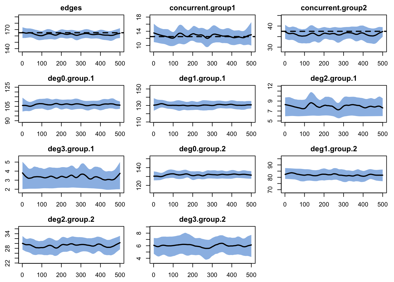
One might want to do a full tergm estimation instead of the approximation. But it is important to consider your goals, and both the relative and absolute magnitude of the bias here. For our purposes, this fit is good enough to move forward.

24.3 Epidemic Model

For the disease simulation, we will simulate an SIR epidemic in a closed population.

24.3.1 Parameterization

The epidemic model parameters are below. In this tutorial, we will use biological parameters for the infection probability per act and recovery rates as equal to demonstrate the impact of group-specific degree distributions on outcomes. Note that the group-specific parameters for the infection probability govern the risk of infection to persons in that group given contact with persons in the other group.

param <- param.net(inf.prob = 0.3, inf.prob.g2 = 0.3,
                   rec.rate = 0.02, rec.rate.g2 = 0.02)

At the outset, 10 people in each group will be infected. For an SIR epidemic simulation, it is necessary to specify the number recovered in each group, here starting at 0.

init <- init.net(i.num = 10, i.num.g2 = 10, 
                 r.num = 0, r.num.g2 = 0)

For control settings, we will simulate 5 epidemics over 500 time steps each. Here we use the multi-core functionality in our controls.

control <- control.net(type = "SIR", nsims = 5, nsteps = 500, ncores = 5)

24.3.2 Simulation

The model is simulated by inputting the fitted network model, the epidemic parameters, the initial conditions, and control settings.

sim <- netsim(est, param, init, control)

Printing the model object shows the inputs and outputs from the simulation object. In particular, take note of the Variables listing; the epidemic outputs for Group 1 are listed without a suffix whereas the outputs for Group 2 are listed with a .g2 suffix.

sim

EpiModel Simulation
=======================
Model class: netsim

Simulation Summary
-----------------------
Model type: SIR
No. simulations: 5
No. time steps: 500
No. NW groups: 2

Fixed Parameters
---------------------------
inf.prob = 0.3
rec.rate = 0.02
inf.prob.g2 = 0.3
rec.rate.g2 = 0.02
act.rate = 1
groups = 2

Model Output
-----------------------
Variables: s.num i.num r.num num s.num.g2 i.num.g2 
r.num.g2 num.g2 si.flow si.flow.g2 ir.flow ir.flow.g2
Networks: sim1 ... sim5
Transmissions: sim1 ... sim5

Formation Statistics
----------------------- 
                  Target Sim Mean Pct Diff Sim SE Z Score SD(Sim Means)
edges              165.0  163.797   -0.729  1.024  -1.175         2.059
nodematch.group      0.0    0.000      NaN    NaN     NaN         0.000
concurrent.group1   12.5   13.086    4.691  0.402   1.460         0.820
concurrent.group2   37.5   36.725   -2.067  0.364  -2.129         0.494
                  SD(Statistic)
edges                    10.829
nodematch.group           0.000
concurrent.group1         3.593
concurrent.group2         4.726


Duration Statistics
----------------------- 
      Target Sim Mean Pct Diff Sim SE Z Score SD(Sim Means) SD(Statistic)
edges     20   20.136    0.678  0.156   0.868         0.368         1.458

Dissolution Statistics
----------------------- 
      Target Sim Mean Pct Diff Sim SE Z Score SD(Sim Means) SD(Statistic)
edges   0.05     0.05   -0.716      0  -1.094         0.001         0.017

24.3.3 Analysis

Similar to the first tutorial, plotting the netsim object shows the prevalence for each disease state in the model over time.

par(mfrow = c(1, 1))
plot(sim, main = "Disease State Sizes")

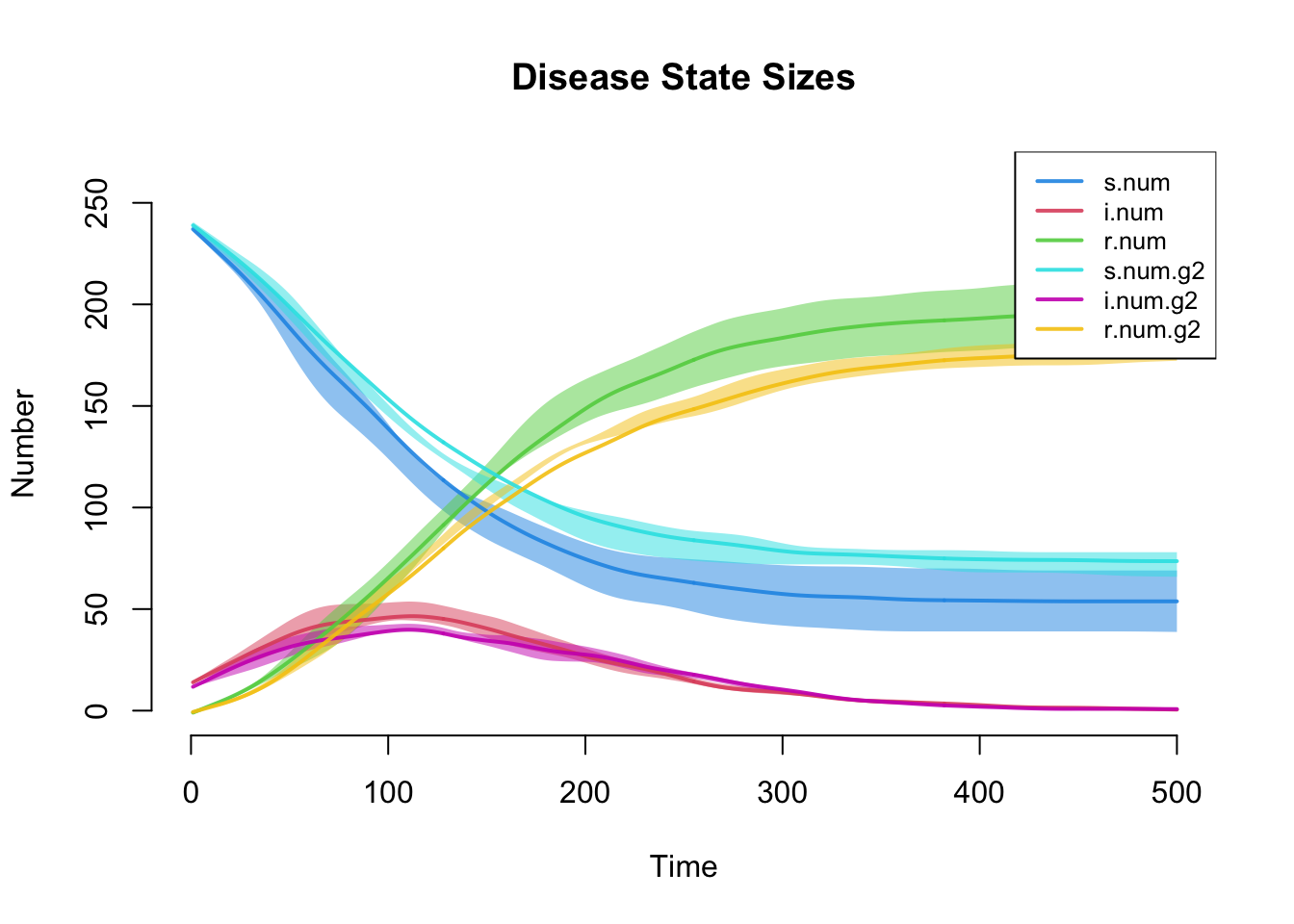
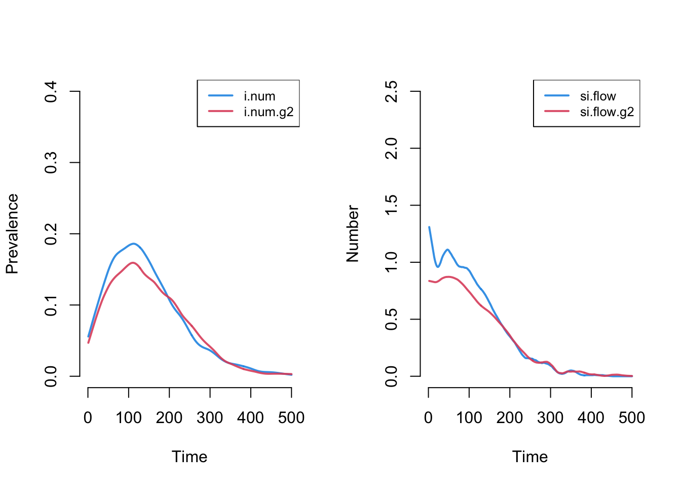
The plot below more clearly shows prevalence and incidence by group Interestingly, women (Group 1) have a slightly higher prevalence of disease during the main epidemic period, and more women than men end up in the recovered state. Men and women have the same mean degree but men have a higher prevalence of concurrency (degree 2+) than women. Following epidemiological and network theory, conditional on mean degree (which is the same for both groups in this model), concurrency increases the risk of transmission but not acquisition. So therefore, women bear the higher burden of male concurrency.

par(mfrow = c(1,2))
plot(sim, y = c("i.num", "i.num.g2"), popfrac = TRUE,
     qnts = FALSE, ylim = c(0, 0.4), legend = TRUE)
plot(sim, y = c("si.flow", "si.flow.g2"), 
     qnts = FALSE, ylim = c(0, 2.5), legend = TRUE)

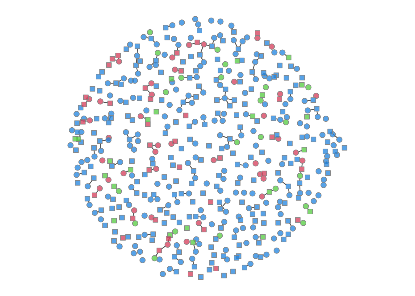
It is possible to plot the color-coded static network at various time points during the simulation, as in the last tutorial. This helps to visualize how womens’ (circle) risk is dependent on their male (square) partners’ network connections.

par(mfrow = c(1, 1), mar = c(0, 0, 0, 0))
plot(sim, type = "network", col.status = TRUE, at = 50, 
     sims = "mean", shp.g2 = "square")

It is possible to add new variables to an existing model object with mutate_epi, which takes inspiration from the mutate functions in the tidyverse. With a time step unit of a week, we can calculate standardized incidence rates per 100 person-years at risk using the following approach. The mutate_epi function takes a netsim object and adds a new variable.

sim <- mutate_epi(sim, ir.g1 = (si.flow / s.num) * 100 * 52,
                       ir.g2 = (si.flow.g2 / s.num.g2) * 100 * 52)

Printing out the object, you can see that these two new variables are in the variable list.

sim

EpiModel Simulation
=======================
Model class: netsim

Simulation Summary
-----------------------
Model type: SIR
No. simulations: 5
No. time steps: 500
No. NW groups: 2

Fixed Parameters
---------------------------
inf.prob = 0.3
rec.rate = 0.02
inf.prob.g2 = 0.3
rec.rate.g2 = 0.02
act.rate = 1
groups = 2

Model Output
-----------------------
Variables: s.num i.num r.num num s.num.g2 i.num.g2 
r.num.g2 num.g2 si.flow si.flow.g2 ir.flow ir.flow.g2 ir.g1 
ir.g2
Networks: sim1 ... sim5
Transmissions: sim1 ... sim5

Formation Statistics
----------------------- 
                  Target Sim Mean Pct Diff Sim SE Z Score SD(Sim Means)
edges              165.0  163.797   -0.729  1.024  -1.175         2.059
nodematch.group      0.0    0.000      NaN    NaN     NaN         0.000
concurrent.group1   12.5   13.086    4.691  0.402   1.460         0.820
concurrent.group2   37.5   36.725   -2.067  0.364  -2.129         0.494
                  SD(Statistic)
edges                    10.829
nodematch.group           0.000
concurrent.group1         3.593
concurrent.group2         4.726


Duration Statistics
----------------------- 
      Target Sim Mean Pct Diff Sim SE Z Score SD(Sim Means) SD(Statistic)
edges     20   20.136    0.678  0.156   0.868         0.368         1.458

Dissolution Statistics
----------------------- 
      Target Sim Mean Pct Diff Sim SE Z Score SD(Sim Means) SD(Statistic)
edges   0.05     0.05   -0.716      0  -1.094         0.001         0.017

After we add the new variable, we can plot and analyze it like any other built-in variable.

par(mar = c(3,3,2,1))
plot(sim, y = c("ir.g1", "ir.g2"), legend = TRUE,
     main = "Standardized Incidence Rates by Group")

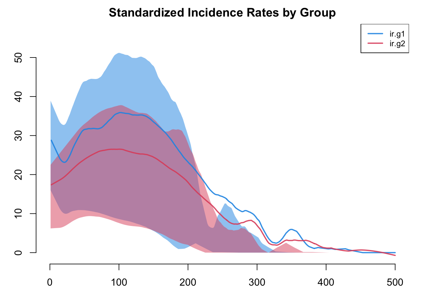
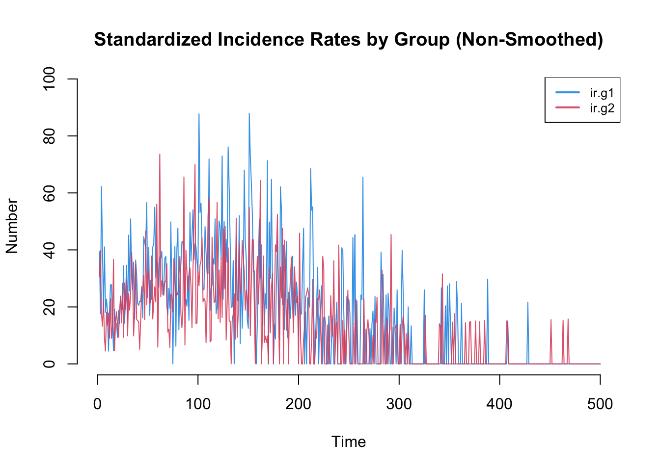
Incidence rates in particular are often highly variable. The plot by default will use a loess smoother so some of this variability may be lost. Therefore, it is worth inspecting the non-smoothed plots too.

plot(sim, y = c("ir.g1", "ir.g2"), legend = TRUE, 
     mean.smooth = FALSE, qnts = FALSE, mean.lwd = 1,
     main = "Standardized Incidence Rates by Group (Non-Smoothed)")

As another exercise, let’s extract the data into a data frame and then calculate some other relevant summary statistics. By default as.data.frame will extract the individual simulation data in each row, but by specifying out = "mean" we can see the time specific averages for all the variables across simulations. The variables in this data frame include both the original variables from netsim plus the two new ones we added with mutate_epi.

df <- as.data.frame(sim, out = "mean")
head(df, 10)

   time s.num i.num r.num num s.num.g2 i.num.g2 r.num.g2 num.g2 si.flow
1     1 240.0  10.0   0.0 250    240.0     10.0      0.0    250     NaN
2     2 238.2  11.6   0.2 250    238.6     11.4      0.0    250     1.8
3     3 237.4  12.2   0.4 250    236.8     13.2      0.0    250     0.8
4     4 234.6  14.8   0.6 250    236.0     14.0      0.0    250     2.8
5     5 232.8  16.2   1.0 250    235.4     14.6      0.0    250     1.8
6     6 232.0  17.0   1.0 250    234.4     15.0      0.6    250     0.8
7     7 230.2  18.8   1.0 250    234.0     15.2      0.8    250     1.8
8     8 229.4  19.6   1.0 250    233.8     15.2      1.0    250     0.8
9     9 228.4  20.0   1.6 250    233.0     15.6      1.4    250     1.0
10   10 227.6  20.2   2.2 250    232.4     16.0      1.6    250     0.8
   si.flow.g2 ir.flow ir.flow.g2    ir.g1     ir.g2
1         NaN     NaN        NaN      NaN       NaN
2         1.4     0.2        0.0 39.34648 30.606982
3         1.8     0.2        0.0 17.59009 39.812782
4         0.8     0.2        0.0 62.24358 17.684335
5         0.6     0.4        0.0 40.69872 13.240047
6         1.0     0.0        0.6 17.93170 22.224826
7         0.4     0.0        0.2 41.04502  8.927203
8         0.2     0.0        0.2 18.10826  4.521739
9         0.8     0.6        0.4 22.75234 18.166285
10        0.6     0.6        0.2 18.45234 13.586502

One interesting summary statistic for an SIR epidemic is the cumulative incidence. Here are the mean cumulative incidences in the first and second groups across simulations. It is necessary here to use na.rm = TRUE to calculate these statistics by removing the first row where the value is undefined.

sum(df$si.flow, na.rm = TRUE)

[1] 186.2

sum(df$si.flow.g2, na.rm = TRUE)

[1] 166.4

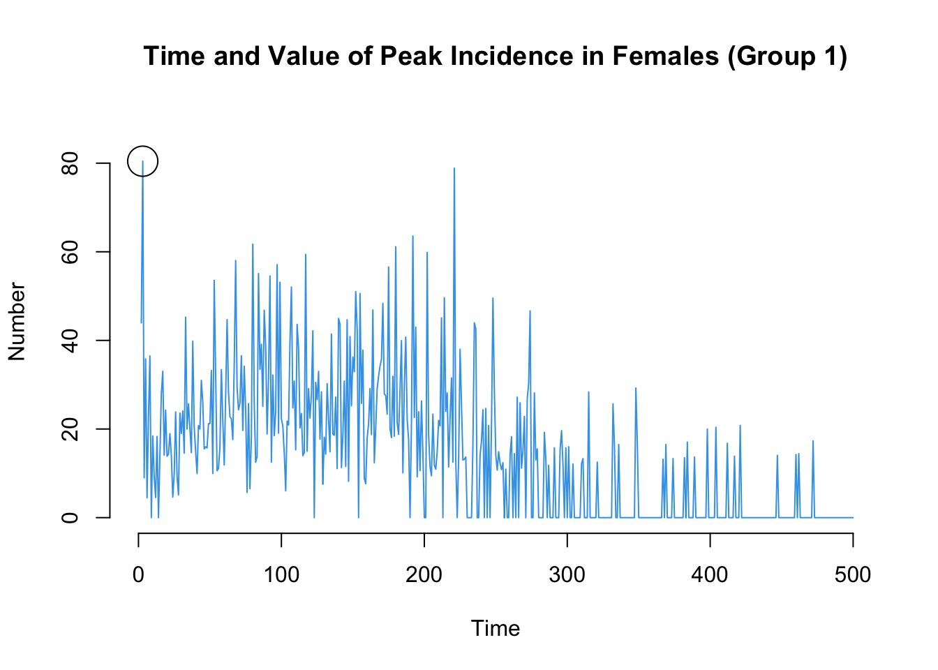
Here are two more that may be of interest: the time point of the peak standardized incidence rates, and also the value of the incidence rate at that time point.

which.max(df$ir.g1)

[1] 151

df$ir.g1[which.max(df$ir.g1)]

[1] 87.94118

plot(sim, y = "ir.g1",
     mean.smooth = FALSE, qnts = FALSE, mean.lwd = 1,
     main = "Time and Value of Peak Incidence in Females (Group 1)")
points(which.max(df$ir.g1), df$ir.g1[which.max(df$ir.g1)], cex = 3)

The transmission matrix again shows the individual transmission events that occurred at each time step, along with information about the infecting partner that may be relevant.

tm <- get_transmat(sim)
head(tm, 10)

# A tibble: 10 × 8
# Groups:   at, sus [10]
      at   sus   inf network infDur transProb actRate finalProb
   <dbl> <int> <int>   <int>  <dbl>     <dbl>   <dbl>     <dbl>
 1     2    98   418       1     50       0.3       1       0.3
 2     2   137   482       1    132       0.3       1       0.3
 3     2   243   332       1     79       0.3       1       0.3
 4     2   317   238       1     69       0.3       1       0.3
 5     2   402   234       1     53       0.3       1       0.3
 6     4    41   317       1      2       0.3       1       0.3
 7     4    52   459       1     12       0.3       1       0.3
 8     4    79   482       1    134       0.3       1       0.3
 9     4   161   418       1     52       0.3       1       0.3
10     4   215   263       1     12       0.3       1       0.3

The infDur column shows the duration of infection (in time steps) of the infecting partner at the point of transmission. For example, an event with an infDur of 1 means that the infecting partner had just become infected themselves in the prior time step. This is the proportion of transmission that occurred in that state.

mean(tm$infDur == 1)

[1] 0.07853403

One can also convert this into a phylogeny for easier visualization of these transmission chains. First, we convert the transmission matrix into a phylo class object that can then be further analyzed and visualized with the ape package. In this transmission matrix, there are multiple trees found because we seeded the infection with 20 people as initial conditions.

tmPhylo <- as.phylo.transmat(tm)

found multiple trees, returning a list of 15phylo objects

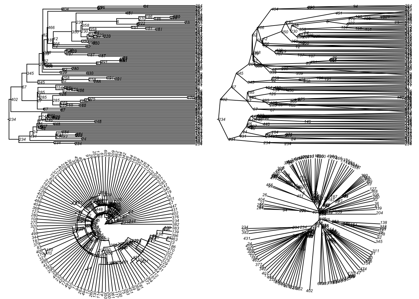
Here is a standard phylogram of the first four trees. Some initial seeds lead to many downstream infections whereas others do not. Is this a function of underlying contact networks of the seeded nodes, the biology or behavior of those nodes, or something else? This could all be tested!

par(mfrow = c(2, 2), mar = c(0, 0, 0, 0))
plot(tmPhylo[[1]], show.node.label = TRUE, root.edge = TRUE, cex = 0.5)
plot(tmPhylo[[2]], show.node.label = TRUE, root.edge = TRUE, cex = 0.5)
plot(tmPhylo[[3]], show.node.label = TRUE, root.edge = TRUE, cex = 0.5)
plot(tmPhylo[[4]], show.node.label = TRUE, root.edge = TRUE, cex = 0.5)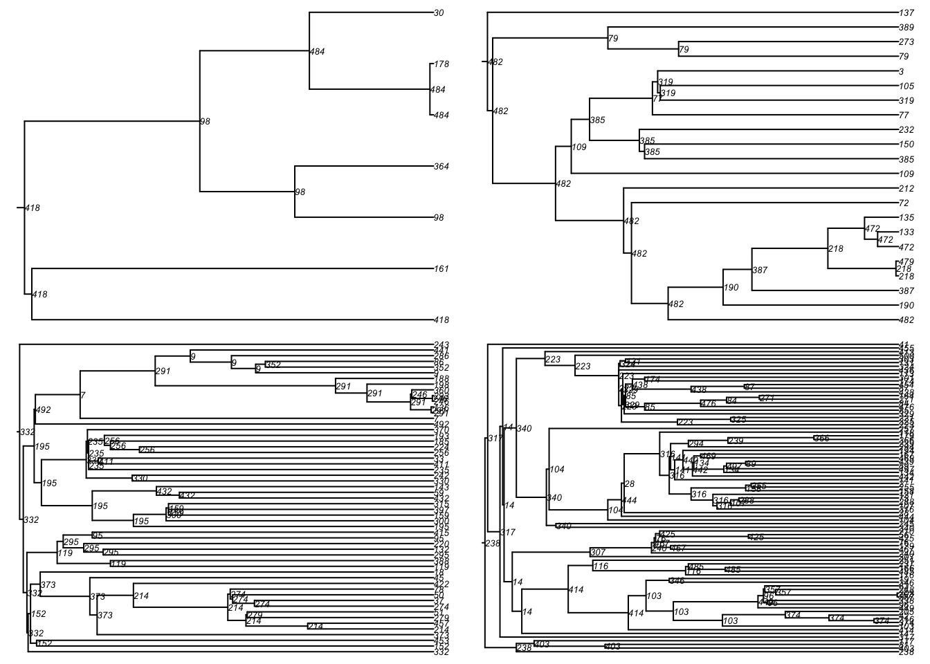

In phylo objects with multiple trees, each tree is stored with a named object. Note that these names correspond to the ID numbers in the transmission matrix itself. We can extract one tree like so:

names(tmPhylo)

 [1] "seed_418" "seed_482" "seed_332" "seed_238" "seed_234" "seed_459"
 [7] "seed_263" "seed_5"   "seed_331" "seed_445" "seed_197" "seed_252"
[13] "seed_168" "seed_211" "seed_471"

tmPhylo5 <- tmPhylo[[5]]

Then we can plot that particular tree as a phylogram and other visual types included in the ape package.

par(mfrow = c(2, 2), mar = c(0, 0, 0, 0))
plot(tmPhylo5, type = "phylogram",
     show.node.label = TRUE, root.edge = TRUE, cex = 0.5)
plot(tmPhylo5, type = "cladogram",
     show.node.label = TRUE, root.edge = TRUE, cex = 0.5)
plot(tmPhylo5, type = "fan",
     show.node.label = TRUE, root.edge = TRUE, cex = 0.5)
plot(tmPhylo5, type = "unrooted",
     show.node.label = TRUE, root.edge = TRUE, cex = 0.5)