43 Modeling an Epidemic on a Multi-Layer Network

This tutorial demonstrates the functionality of representing and simulating an epidemic on a multi-layer network in EpiModel. The set of nodes must be the same for all networks. This model will include two layers in which there is interaction between the two layers. Specifically, the degree in one network will be used as a model term in the other network to allow for negative correlation in degree across the two layers. Additionally, the mean duration of relationships in the two network layers will differ.

Note

Download the R script to follow along with this tutorial here.

43.1 Setup

First start by loading EpiModel and clearing your global environment.

Code

library(EpiModel)
rm(list = ls())

43.2 Model Goals

Our goal for this exercise will be to model two dependent layers of a network, with different additional network configuration terms in each network. The layer dependency will emerge with a nodefactor term in which the degree of network 1 will depend on the degree (specifically having a degree of 1+) in network 2, and vice versa. Additional terms in layer 1 are assortative mixing by race, handled with a nodematch term; and for layer 2 are a degree(1) term that controls that aspect of the degree distribution. In summary, for multi-layer networks, we can have different models for formation (and dissolution) and interactions between layers.

Code

formation.1 <- ~edges + nodematch("race") + nodefactor("deg1+.net2")
formation.2 <- ~edges + degree(1) + nodefactor("deg1+.net1")

Here are the target statistics for our two models. As shown below, mean degree is lower in layer 2 than in layer 1. The final target stats in each vector are controlling the cross-layer nodefactor terms. As we will see below, the small values of those target stats will result in a strong negative correlation between mean degree across layers (having relations in layer 1 makes one less likely to have relations in layer 2).

Code

target.stats.1 <- c(90, 60, 10)
target.stats.2 <- c(75, 120, 10)

In addition to differences in the formation models, there will be a key difference in the dissolution model: the average relational duration in layer 2 will be shorter than that in layer 1.

Code

coef.diss.1 <- dissolution_coefs(dissolution = ~offset(edges), duration = 100)
coef.diss.2 <- dissolution_coefs(dissolution = ~offset(edges), duration = 75)

43.3 Network Setup

Ok, now, we need to go back and start setting up the network. Because there are cross-layer interactions, this will be a little more complex than usual. We first start by setting up an empty network of 500 nodes, and then add a demographic attribute (race) that is binary.

Code

nw <- network_initialize(500)
nw <- set_vertex_attribute(nw, "race", rep(0:1, length.out = 500))

Next, because we will include degree as an ERGM term across network layers, we will use the san function in the ergm package to create good starting values of degree in each of the network. The san function uses a “simulated annealing” algorithm to simulate edge sets that are consistent with dyad-independent formulas. First, we start with generating a network with edges and nodematch terms to generate an edgeset consistent with overall mean degree and race homophily.

Code

nw_san <- san(nw ~ edges + nodematch("race"), target.stats = c(90, 60))
nw_san

 Network attributes:
  vertices = 500 
  directed = FALSE 
  hyper = FALSE 
  loops = FALSE 
  multiple = FALSE 
  bipartite = FALSE 
  total edges= 90 
    missing edges= 0 
    non-missing edges= 90 

 Vertex attribute names: 
    race vertex.names 

No edge attributes

We can see the estimated degree for each node in the network with get_degree.

Code

get_degree(nw_san)

  [1] 0 0 0 0 1 3 0 1 0 0 1 0 1 0 2 1 0 2 0 0 0 3 1 1 0 0 0 1 2 1 0 0 0 0 1 1 1
 [38] 0 0 1 0 1 0 0 0 0 0 0 0 1 0 0 0 0 0 0 0 0 1 0 0 0 0 0 0 1 1 0 2 2 0 2 2 0
 [75] 0 2 1 1 0 0 1 0 0 1 1 0 0 0 0 0 1 1 1 0 0 0 0 0 1 0 0 0 0 3 0 0 1 0 0 0 0
[112] 3 1 0 1 1 1 0 0 0 0 0 0 0 1 0 0 2 0 0 0 1 1 0 0 0 0 2 1 0 0 0 1 0 0 0 0 1
[149] 1 0 3 1 0 0 0 0 0 0 1 0 1 0 0 0 0 1 0 0 0 0 1 0 0 1 0 0 1 1 0 0 1 0 0 0 0
[186] 0 0 0 1 0 0 0 0 0 0 1 0 0 0 1 1 2 1 0 0 1 0 4 0 1 0 0 0 0 0 0 0 0 0 0 0 0
[223] 0 0 0 0 0 0 0 0 0 0 0 1 0 0 0 0 1 0 0 0 1 0 1 0 1 0 0 0 0 0 0 0 1 1 1 0 0
[260] 0 0 0 1 0 0 1 0 1 1 0 1 0 0 0 0 0 1 1 0 0 0 0 0 0 0 0 0 0 0 0 0 0 1 2 0 2
[297] 0 0 0 0 1 0 0 1 2 0 0 0 1 0 0 0 0 2 2 0 0 0 1 0 0 1 0 0 0 0 0 0 0 0 0 0 1
[334] 2 0 1 0 0 2 1 1 0 0 0 0 0 1 0 0 0 0 1 0 0 1 0 0 1 0 0 0 0 1 0 0 0 0 2 0 0
[371] 0 0 0 2 1 0 1 0 0 0 0 2 0 0 0 0 0 0 0 0 0 0 0 0 0 0 0 0 1 1 0 1 0 0 0 0 0
[408] 1 1 0 0 0 0 1 0 0 0 0 0 0 1 0 0 0 0 0 0 0 0 0 0 0 0 0 0 1 0 0 2 0 0 0 0 0
[445] 1 0 0 1 0 1 0 0 1 0 0 0 0 1 1 0 0 0 0 0 1 1 0 0 0 0 0 0 0 0 0 0 0 1 0 0 0
[482] 1 0 1 1 1 2 1 1 0 0 0 0 2 0 0 1 0 1 1

Next, we set network degree on the network with set_vertex_attribute called deg.net1.

Code

nw_san <- set_vertex_attribute(nw_san, "deg.net1", get_degree(nw_san))

We can also use a categorical (binary) transformation of continuous degree, called deg1+.net1, for having a degree of 1 or more.

Code

nw_san <- set_vertex_attribute(nw_san, "deg1+.net1",
                               pmin(get_degree(nw_san), 1))

Next, we use san again to create a network for the second layer that follows the main model terms plus the target statistic for the cross-layer effect. Again, we will use a binary categorization for the degree, with a cut-point of 1+. Then we set that degree value as an attribute on the network.

Code

nw_san_2 <- san(nw_san ~ edges + degree(1) + nodefactor("deg1+.net1")
                  + Sum(matrix(seq_len(network.size(nw)), nrow = 1) ~
                        degrange(1, by = "deg.net1", levels = -1),label="Sum"),
                target.stats = c(75, 120, 10, 10))
nw_san <- set_vertex_attribute(nw_san, "deg1+.net2", pmin(get_degree(nw_san_2), 1))

Next, we confirm that we have come close to our intended targets for both network layers. These do not need to be perfect, as they are just starting conditions for further estimating the model in ergm.

Code

summary(nw_san ~ edges + nodematch("race") + nodefactor("deg1+.net2"))

                  edges          nodematch.race nodefactor.deg1+.net2.1 
                     90                      60                      10

Code

summary(nw_san_2 ~ edges + degree(1) + nodefactor("deg1+.net1"))

                  edges                 degree1 nodefactor.deg1+.net1.1 
                     75                     120                      10

As the final step before model estimation, we set the binary network degree attributes for each network as attributes on the original nw object.

Code

nw <- set_vertex_attribute(nw, "deg1+.net1", pmin(get_degree(nw_san), 1))
nw <- set_vertex_attribute(nw, "deg1+.net2", pmin(get_degree(nw_san_2), 1))

43.4 Network Model Estimation

Here is the definition of the formation component of the models again.

Code

formation.1 <- ~edges + nodematch("race") + nodefactor("deg1+.net2")
formation.2 <- ~edges + degree(1) + nodefactor("deg1+.net1")

And here are the target statistics again for each term in each layer.

Code

target.stats.1 <- c(90, 60, 10)
target.stats.2 <- c(75, 120, 10)

And here is the definition of the dissolution models again.

Code

coef.diss.1 <- dissolution_coefs(dissolution = ~offset(edges), duration = 100)
coef.diss.2 <- dissolution_coefs(dissolution = ~offset(edges), duration = 75)

Finally, we fit the models. Even though we conceptually think of this as one multi-layer network, in fact we are modeling with two separate network models that have a link through their model terms. Therefore, we have two calls to netest and two model objects to keep.

Code

est.1 <- netest(nw, formation.1, target.stats.1, coef.diss.1,
                set.control.ergm = ergm::control.ergm(
                  main.method = "MCMLE",
                  MCMLE.maxit = 500,
                  SAN.maxit = 3,
                  SAN.nsteps.times = 4,
                  MCMC.samplesize = 1e4,
                  MCMC.interval = 5e3,
                ))
est.2 <- netest(nw, formation.2, target.stats.2, coef.diss.2,
                set.control.ergm = ergm::control.ergm(
                  main.method = "MCMLE",
                  MCMLE.maxit = 500,
                  SAN.maxit = 3,
                  SAN.nsteps.times = 4,
                  MCMC.samplesize = 1e4,
                  MCMC.interval = 5e3,
                ))

Let’s take a look at the model coefficients for the two netest objects. The coefficients for layer 1 show a strong negative coefficient for the cross-degree term, suggesting there will be many fewer layer 1 contacts if there are any layer 2 contacts.

Code

summary(est.1)

Call:
ergm(formula = formation, constraints = constraints, offset.coef = coef.form, 
    target.stats = target.stats, eval.loglik = FALSE, control = set.control.ergm, 
    verbose = verbose, basis = nw)

Maximum Likelihood Results:

                        Estimate Std. Error MCMC % z value Pr(>|z|)    
edges                    -7.1307     0.1862      0 -38.299   <1e-04 ***
nodematch.race            0.6982     0.2237      0   3.121   0.0018 ** 
nodefactor.deg1+.net2.1  -1.8319     0.3256      0  -5.627   <1e-04 ***
---
Signif. codes:  0 '***' 0.001 '**' 0.01 '*' 0.05 '.' 0.1 ' ' 1

Log-likelihood was not estimated for this fit. To get deviances, AIC, and/or BIC, use ‘*fit* <-logLik(*fit*, add=TRUE)’ to add it to the object or rerun this function with eval.loglik=TRUE.


Dissolution Coefficients
=======================
Dissolution Model: ~offset(edges)
Target Statistics: 100
Crude Coefficient: 4.59512
Mortality/Exit Rate: 0
Adjusted Coefficient: 4.59512

And there is a similarly signed coefficient for layer 2.

Code

summary(est.2)

Call:
ergm(formula = formation, constraints = constraints, offset.coef = coef.form, 
    target.stats = target.stats, eval.loglik = FALSE, control = set.control.ergm, 
    verbose = verbose, basis = nw)

Monte Carlo Maximum Likelihood Results:

                        Estimate Std. Error MCMC % z value Pr(>|z|)    
edges                    -7.2337     0.2272      0 -31.833   <1e-04 ***
degree1                   0.3684     0.1584      0   2.325   0.0201 *  
nodefactor.deg1+.net1.1  -1.8792     0.3423      0  -5.490   <1e-04 ***
---
Signif. codes:  0 '***' 0.001 '**' 0.01 '*' 0.05 '.' 0.1 ' ' 1

Log-likelihood was not estimated for this fit. To get deviances, AIC, and/or BIC, use ‘*fit* <-logLik(*fit*, add=TRUE)’ to add it to the object or rerun this function with eval.loglik=TRUE.


Dissolution Coefficients
=======================
Dissolution Model: ~offset(edges)
Target Statistics: 75
Crude Coefficient: 4.304065
Mortality/Exit Rate: 0
Adjusted Coefficient: 4.304065

43.5 Model Diagnostics

Next we run the model diagnostics.

Code

dx.1 <- netdx(est.1, nsims = 25, ncores = 5, nsteps = 1000)


Network Diagnostics
-----------------------
- Simulating 25 networks
- Calculating formation statistics

We need to run these for each network layer separately. Because the network size is relatively small and some of the values of the target statistics is also small, we run lots of simulations of the network. In general, model diagnostics are acceptable for layer 1.

Code

print(dx.1)

EpiModel Network Diagnostics
=======================
Diagnostic Method: Dynamic
Simulations: 25
Time Steps per Sim: 1000

Formation Diagnostics
----------------------- 
                        Target Sim Mean Pct Diff Sim SE Z Score SD(Sim Means)
edges                       90   89.895   -0.116  0.654  -0.160         3.487
nodematch.race              60   59.724   -0.459  0.560  -0.493         3.098
nodefactor.deg1+.net2.1     10    9.892   -1.080  0.202  -0.535         1.132
                        SD(Statistic)
edges                           9.278
nodematch.race                  7.664
nodefactor.deg1+.net2.1         2.991

Duration Diagnostics
----------------------- 
      Target Sim Mean Pct Diff Sim SE Z Score SD(Sim Means) SD(Statistic)
edges    100   98.766   -1.234   0.73  -1.691         3.376        10.156

Dissolution Diagnostics
----------------------- 
      Target Sim Mean Pct Diff Sim SE Z Score SD(Sim Means) SD(Statistic)
edges   0.01     0.01    0.577      0   0.856             0         0.011

Code

plot(dx.1, plots.joined = FALSE, mean.smooth = FALSE)

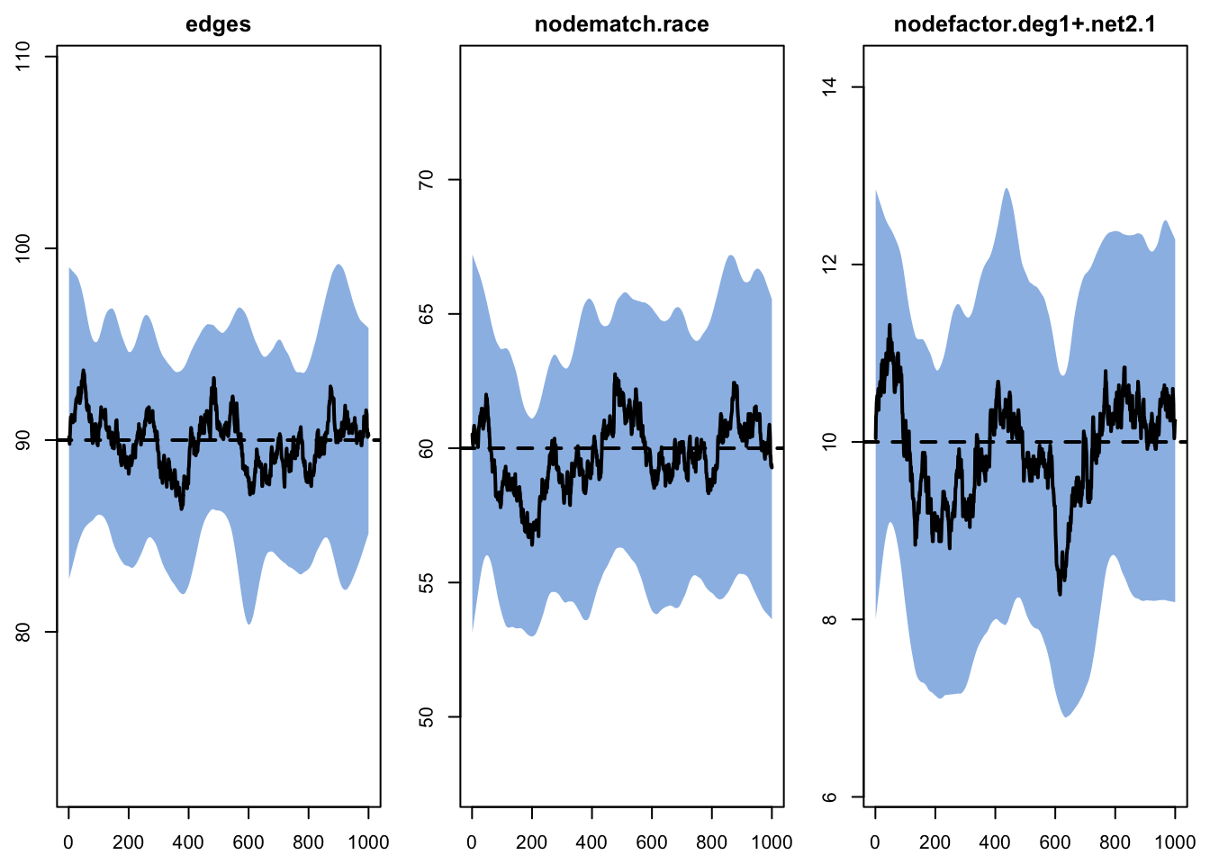
Next, we run model diagnostics for network layer 2.

Code

dx.2 <- netdx(est.2, nsims = 25, ncores = 5, nsteps = 1000)


Network Diagnostics
-----------------------
- Simulating 25 networks
- Calculating formation statistics

Model diagnostics for network layer 2. Model diagnostics are acceptable for this layer too.

Code

print(dx.2)

EpiModel Network Diagnostics
=======================
Diagnostic Method: Dynamic
Simulations: 25
Time Steps per Sim: 1000

Formation Diagnostics
----------------------- 
                        Target Sim Mean Pct Diff Sim SE Z Score SD(Sim Means)
edges                       75   75.316    0.422  0.452   0.700         2.606
degree1                    120  120.559    0.466  0.643   0.870         3.215
nodefactor.deg1+.net1.1     10    9.512   -4.883  0.218  -2.242         1.338
                        SD(Statistic)
edges                           7.830
degree1                        11.572
nodefactor.deg1+.net1.1         3.325

Duration Diagnostics
----------------------- 
      Target Sim Mean Pct Diff Sim SE Z Score SD(Sim Means) SD(Statistic)
edges     75   75.187     0.25  0.549   0.342         2.965         8.722

Dissolution Diagnostics
----------------------- 
      Target Sim Mean Pct Diff Sim SE Z Score SD(Sim Means) SD(Statistic)
edges  0.013    0.013   -0.149      0  -0.238             0         0.013

Code

plot(dx.2, plots.joined = FALSE, mean.smooth = FALSE)

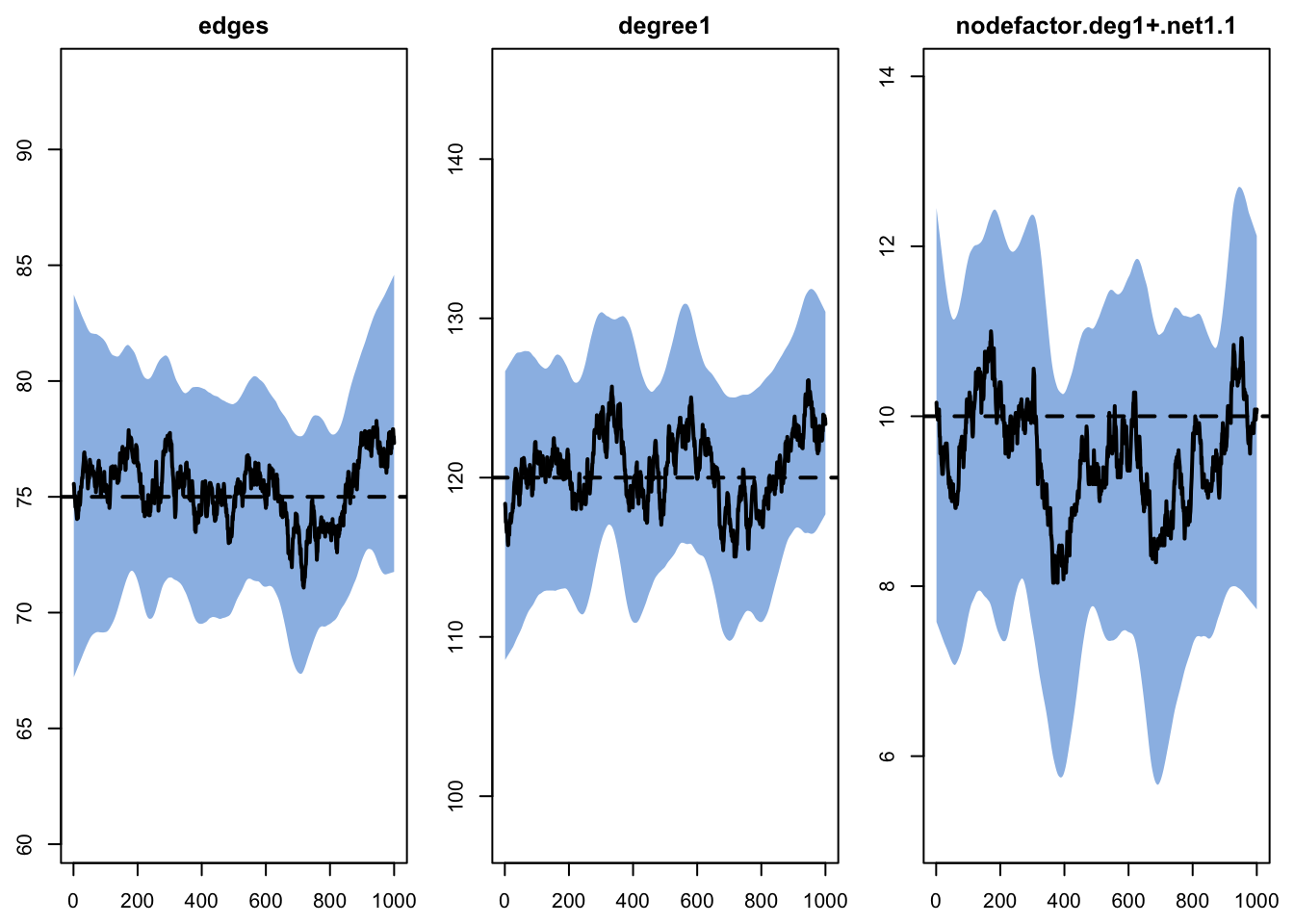
43.6 Epidemic Model Simulation

From here, we can now move on to the epidemic model. We will just run a simple SI model in a closed population to focus on the network aspects of the exercise. Thus, the model parameters and initial conditions are simple

Code

param <- param.net(inf.prob = 0.5, act.rate = 2)
init <- init.net(i.num = 10)

Next, we have to address this problem: mean degree of network layer 1 will depend on the degree of network layer 2 (and vice versa), but the degree of network layer 2 can change stochastically for any given node at any time step. Even though this is a model in a closed population, feedback occurs because the network resimulations for one layer must account for the degree distribution in the other.

Therefore, we need some model code that will be run each time step that performs the following actions: before we simulate layer 1, we need to look up the current degree in layer 2 and update the related nodal attribute; then before we simulate layer 2, we need to look up the current degree in layer 1 and update the related nodal attribute. We also recalculate the layer 2 degree after resimulating layer 2 to get our network summary statistics right. The code below shows how to do this.

Code

network_layer_updates <- function(dat, at, network) {
  if (network == 0) {
    # update deg1+.net2 prior to network 1 simulation,
    # as network 1's formation model depends on this
    # nodal attribute
    dat <- set_attr(dat, "deg1+.net2", pmin(get_degree(dat$run$el[[2]]), 1))
  } else if (network == 1) {
    # update deg1+.net1 prior to network 2 simulation,
    # as network 2's formation model depends on this
    # nodal attribute
    dat <- set_attr(dat, "deg1+.net1", pmin(get_degree(dat$run$el[[1]]), 1))
  } else if (network == 2) {
    # update deg1+.net2 after network 2 simulation,
    # for summary statistics
    dat <- set_attr(dat, "deg1+.net2", pmin(get_degree(dat$run$el[[2]]), 1))
  }
  return(dat)
}

Note the nwstats.formula uses the multilayer function to define the network statistics stats specific to each layer. Note also that we need to make sure that we resimulate the network at each time step with resimulate.network. And note that we pass our network updating function into the workflow with dat.updates.

Code

control <- control.net(type = "SI",
                       nsteps = 500,
                       nsims = 20,
                       ncores = 10,
                       tergmLite = TRUE,
                       resimulate.network = TRUE,
                       set.control.ergm = control.simulate.formula(MCMC.burnin = 4e+05, MCMC.interval = 10000),
                       set.control.tergm = control.simulate.formula.tergm(MCMC.burnin.min = 1e5),
                       dat.updates = network_layer_updates,
                       nwstats.formula = multilayer("formation",
                                                    ~edges + nodefactor("deg1+.net1") + degree(0:4)))

Run the network model simulation with netsim. Note that we pass multiple layers of networks with a list of netest objects.

Code

sim <- netsim(list(est.1, est.2), param, init, control)

43.7 Model Results

Examine the network stats for network layer 1.

Code

print(sim, network = 1)

EpiModel Simulation
=======================
Model class: netsim

Simulation Summary
-----------------------
Model type: SI
No. simulations: 20
No. time steps: 500
No. NW groups: 1

Fixed Parameters
---------------------------
inf.prob = 0.5
act.rate = 2
groups = 1

Model Output
-----------------------
Variables: s.num i.num num si.flow
Networks: sim1 ... sim20
Transmissions: sim1 ... sim20

Formation Statistics
----------------------- 
                        Target Sim Mean Pct Diff Sim SE Z Score SD(Sim Means)
edges                       90   91.910    2.123  0.971   1.967         7.115
nodematch.race              60   61.040    1.733  0.885   1.175         5.418
nodefactor.deg1+.net2.1     10   11.182   11.818  0.296   3.988         2.104
                        SD(Statistic)
edges                          10.647
nodematch.race                  8.594
nodefactor.deg1+.net2.1         4.040


Duration and Dissolution Statistics
----------------------- 
Not available when:
- `control$tergmLite == TRUE`
- `control$save.network == FALSE`
- `control$save.diss.stats == FALSE`
- dissolution formula is not `~ offset(edges)`
- `keep.diss.stats == FALSE` (if merging)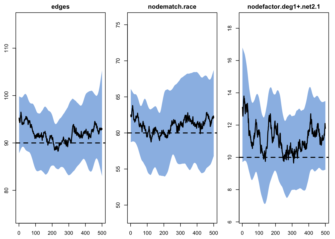

Code

plot(sim, network = 1, type = "formation", plots.joined = FALSE, mean.smooth = FALSE)

Examine the network stats for network layer 2.

Code

print(sim, network = 2)

EpiModel Simulation
=======================
Model class: netsim

Simulation Summary
-----------------------
Model type: SI
No. simulations: 20
No. time steps: 500
No. NW groups: 1

Fixed Parameters
---------------------------
inf.prob = 0.5
act.rate = 2
groups = 1

Model Output
-----------------------
Variables: s.num i.num num si.flow
Networks: sim1 ... sim20
Transmissions: sim1 ... sim20

Formation Statistics
----------------------- 
                        Target Sim Mean Pct Diff Sim SE Z Score SD(Sim Means)
edges                       75   71.559   -4.588  0.730  -4.711         4.345
nodefactor.deg1+.net1.1     10   10.376    3.764  0.265   1.422         1.700
degree0                     NA  371.421       NA  1.142      NA         7.392
degree1                    120  115.346   -3.878  0.901  -5.165         6.399
degree2                     NA   12.024       NA  0.285      NA         1.349
degree3                     NA    1.117       NA  0.064      NA         0.346
degree4                     NA    0.088       NA  0.013      NA         0.068
                        SD(Statistic)
edges                           8.263
nodefactor.deg1+.net1.1         3.513
degree0                        13.413
degree1                        11.717
degree2                         3.918
degree3                         1.097
degree4                         0.293


Duration and Dissolution Statistics
----------------------- 
Not available when:
- `control$tergmLite == TRUE`
- `control$save.network == FALSE`
- `control$save.diss.stats == FALSE`
- dissolution formula is not `~ offset(edges)`
- `keep.diss.stats == FALSE` (if merging)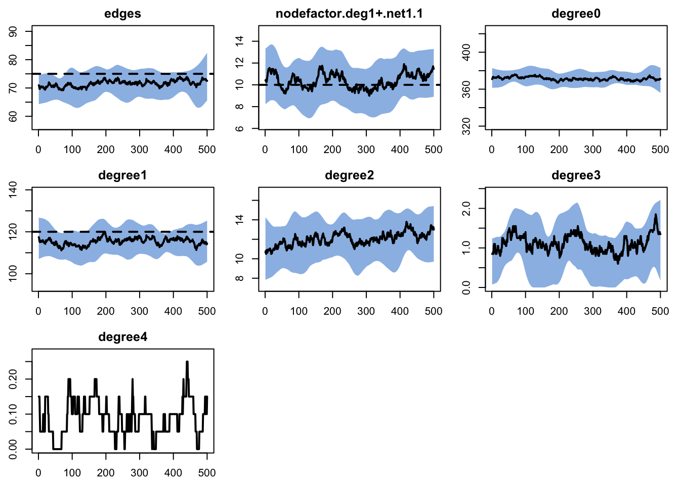

Code

plot(sim, network = 2, type = "formation", plots.joined = FALSE, mean.smooth = FALSE)

There are many more things we can–and do–implement in practice with multilayer networks, but this is how to get started.