34 Lab
In this lab you can explore the impact of using a more detailed model for the Mesa friendship network.
Feel free to explore different specifications, using the ergm function summary(mesa ~ <choose some ergm terms>) to take a look at the \(g(y)\) terms that serve as your target statistics. The great thing about having network census data is that ergm will calculate all of the \(g(y)\) terms for you. So it’s much easier (too easy?) to explore possible specifications, as you don’t need to hand calculate the target statistics.
You can choose to fit any model you like. Below, we explore Model 5 that we fit using statnetWeb in Module 3. Note – it takes a good 5 minutes for the MCMC fit to finish.
Download the R script to follow along with this tutorial here.
First, start by loading the EpiModel, ergm.ego and ndtv packages. Optionally, also install the rglpk package to use the preferred solver during estimation.
Code
data("faux.mesa.high")
mesa <- faux.mesa.high
# model 5 from yesterday: + gwesp
formation <- ~ edges +
nodefactor("Grade") + nodematch("Grade", diff=T) +
nodefactor("Race") + nodematch("Race", diff=T) +
nodefactor("Sex") + nodematch("Sex") +
gwesp(0.5, fixed=T)
targets <- summary(mesa ~ edges +
nodefactor("Grade") + nodematch("Grade", diff=T) +
nodefactor("Race") + nodematch("Race", diff=T) +
nodefactor("Sex") + nodematch("Sex") +
gwesp(0.5, fixed=T))
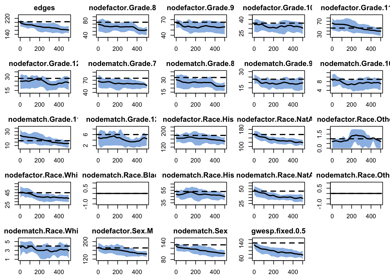
targets edges nodefactor.Grade.8 nodefactor.Grade.9
203.0000 75.0000 65.0000
nodefactor.Grade.10 nodefactor.Grade.11 nodefactor.Grade.12
36.0000 49.0000 28.0000
nodematch.Grade.7 nodematch.Grade.8 nodematch.Grade.9
75.0000 33.0000 23.0000
nodematch.Grade.10 nodematch.Grade.11 nodematch.Grade.12
9.0000 17.0000 6.0000
nodefactor.Race.Hisp nodefactor.Race.NatAm nodefactor.Race.Other
178.0000 156.0000 1.0000
nodefactor.Race.White nodematch.Race.Black nodematch.Race.Hisp
45.0000 0.0000 53.0000
nodematch.Race.NatAm nodematch.Race.Other nodematch.Race.White
46.0000 0.0000 4.0000
nodefactor.Sex.M nodematch.Sex gwesp.fixed.0.5
171.0000 132.0000 141.9258 35 Fit the network model
36 Look at the fit diagnostics
37 Setup the epidemic control parameters
38 Run the epidemic
39 Plot infection prevalence by grade.
Code
mySIS <- mutate_epi(mySIS,
                    prev.7 = i.num.Grade7 / num.Grade7,
                    prev.8 = i.num.Grade8 / num.Grade8,
                    prev.9 = i.num.Grade9 / num.Grade9,
                    prev.10 = i.num.Grade10 / num.Grade10,
                    prev.11 = i.num.Grade11 / num.Grade11,
                    prev.12 = i.num.Grade12 / num.Grade12)

plot(mySIS, y = c("prev.7", "prev.8", "prev.9", "prev.10",
                  "prev.11", "prev.12"),
     qnts.alpha = 0.2, qnts = 0.5,
     main="Prevalence Rate",
     legend = TRUE,
     xlim = c(0,mycontrol$nsteps+25))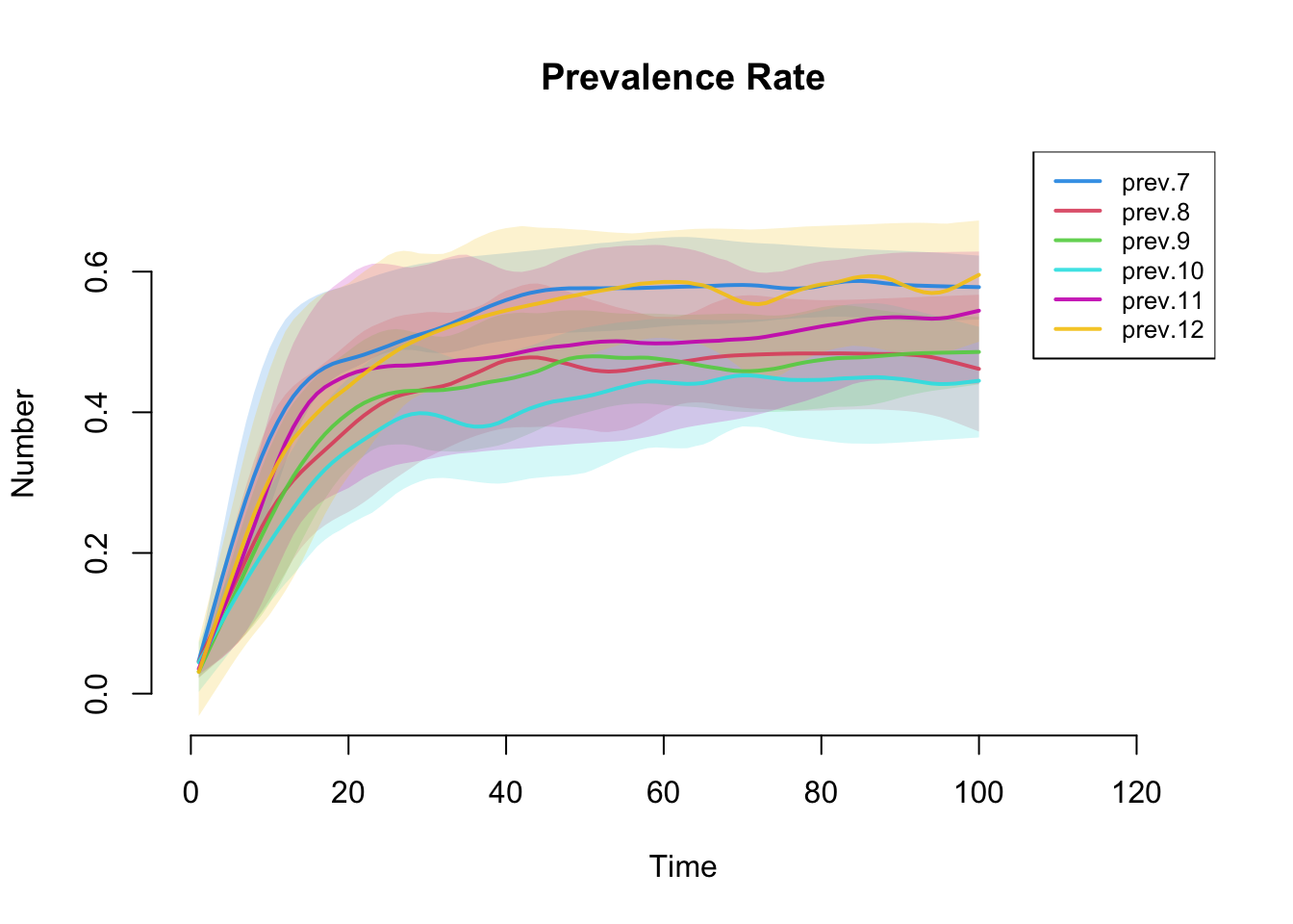
40 Dynamic Visualization
How does this network look, compared to the one produced in the tutorial?
Code
myND <- get_network(mySIS)
myND <- color_tea(myND, verbose = FALSE)

slice.par <- list(start = 1, end = 20, interval = 1,
                  aggregate.dur = 1, rule = "any")
render.par <- list(tween.frames = 10, show.time = FALSE)
plot.par <- list(mar = c(0, 0, 0, 0))

compute.animation(myND, slice.par = slice.par, verbose = TRUE)
render.d3movie(
  myND,
  render.par = render.par,
  plot.par = plot.par,
  vertex.cex = 0.9,
  vertex.col = "ndtvcol",
  edge.col = "darkgrey",
  vertex.border = "lightgrey",
  displaylabels = FALSE,
  output.mode = "htmlWidget")