33 Tutorial
To demonstrate how you can use EpiModel with data inputs from network census and egocentrically sampled designs we will return to the built-in adolescent friendship network data “faux.mesa.high” (“Mesa”) from the ergm package.
We tested and assessed several models for this network yesterday using the
statnetWebshiny app. Here you will learn how to do this from the R command line usingEpiModelpackage syntax.
Mesa is a network census based on one of the “saturation” sample schools from the Add Health study (wave 1). Questionnaires were completed by all of the students from the 7th-12th grades, and they were asked to nominate up to 5 close male and 5 close female friends from a roster that included the names of all students in their school, and a code for friends who were not enrolled in the school. More information on the study design can be found here. The network included in the ergm package is a simplified and anonymized version of the original data, using a model-based simulation of the mutual in-school nominations only, so it is an undirected network. More information on the details and construction of the simulated dataset can be found by typing ?faux.mesa.high.
This is a static network, and the Add Health study did not include questions about partnership duration. We will use a hypothetical average friendship length to parameterize the duration.
Epimodel’s network methods have the flexibility to be entirely driven by a single dataset (when all necessary data have been collected), to combine data from different studies, or to introduce parameters for exploring “what-if” scenarios.
Download the R script to follow along with this tutorial here.
Let’s start by loading the EpiModel package. Optionally, also install the Rglpk package to use the preferred solver during estimation.
33.1 Network Census Data
33.1.1 Load the data
We’ll load it, and as a first step take a look at the class of the object. The class of the built-in Mesa data object is network, which is the type of object you need to pass to a call to ergm. If you have raw data from a network census study design, the methods for creating network objects from your data can be found in one of the Statnet intro workshops.
Next, let’s take a look at the basic network summary. Typing the name of the object prints out a list of the basic properties of the network, properties that are the starting point for considering what types of models can be considered.
 Network attributes:
  vertices = 205
  directed = FALSE
  hyper = FALSE
  loops = FALSE
  multiple = FALSE
  bipartite = FALSE
  total edges= 203
    missing edges= 0
    non-missing edges= 203

 Vertex attribute names:
    Grade Race Sex

No edge attributes
And because our models will condition on the density of our network (or equivalently the mean degree) by using it to construct the null hypothesis expected values of each network statistic, we should look at these two statistics.
- Network density
- Mean degree
Interpretation:
The overall probability of a tie (#ties/#dyads) is about 1% (0.009*100)
On average, students report having about 2 friends.
Note that there is an explicit relationship between density and mean degree (here N is network size, the number of nodes):
\[ Mean Degree = Density * (N-1) \]
(for undirected networks, like we have here – this is slightly different for directed networks)
33.1.2 Explore attribute effects
We’ll focus on two of the attributes here – Grade and Sex – and use some basic R utilities to explore whether these are associated with heterogeneity in behavior (degree) and network structure (mixing patterns).
First, let’s look at the overall degree distribution, and compare it with the BRG null hypothesis values for a network that has this density (or equivalently, this mean degree).
Code
fill.col <- RColorBrewer::brewer.pal(11, "Spectral") # 8 colors
# Overall observed
barplot(degreedist(mesa)/network.size(mesa), xaxt = "n",
main = "Overall degree distribution",
xlab = "Degree", ylab = "Fraction of nodes",
col = "lightblue")
# Bernoulli Random Graph expectation overlay
degs <- gsub("degree", "", names(degreedist(mesa)))
pos <- barplot(degreedist(mesa), plot=F)
axis(1, at = pos, labels = degs)
points(x=pos,
y=dbinom(c(0:10, 13),
size=network.size(mesa),
prob=network.density(mesa)),
col="red", pch=19)
text(10, 0.27,
cex=0.8,
paste("Observed mean degree: ", round(summary(mesa ~ meandeg), 2)))
legend(7.5, 0.25,
cex=0.7, pch=19, col="red", bty="n",
"BRG expected values for observed mean degree")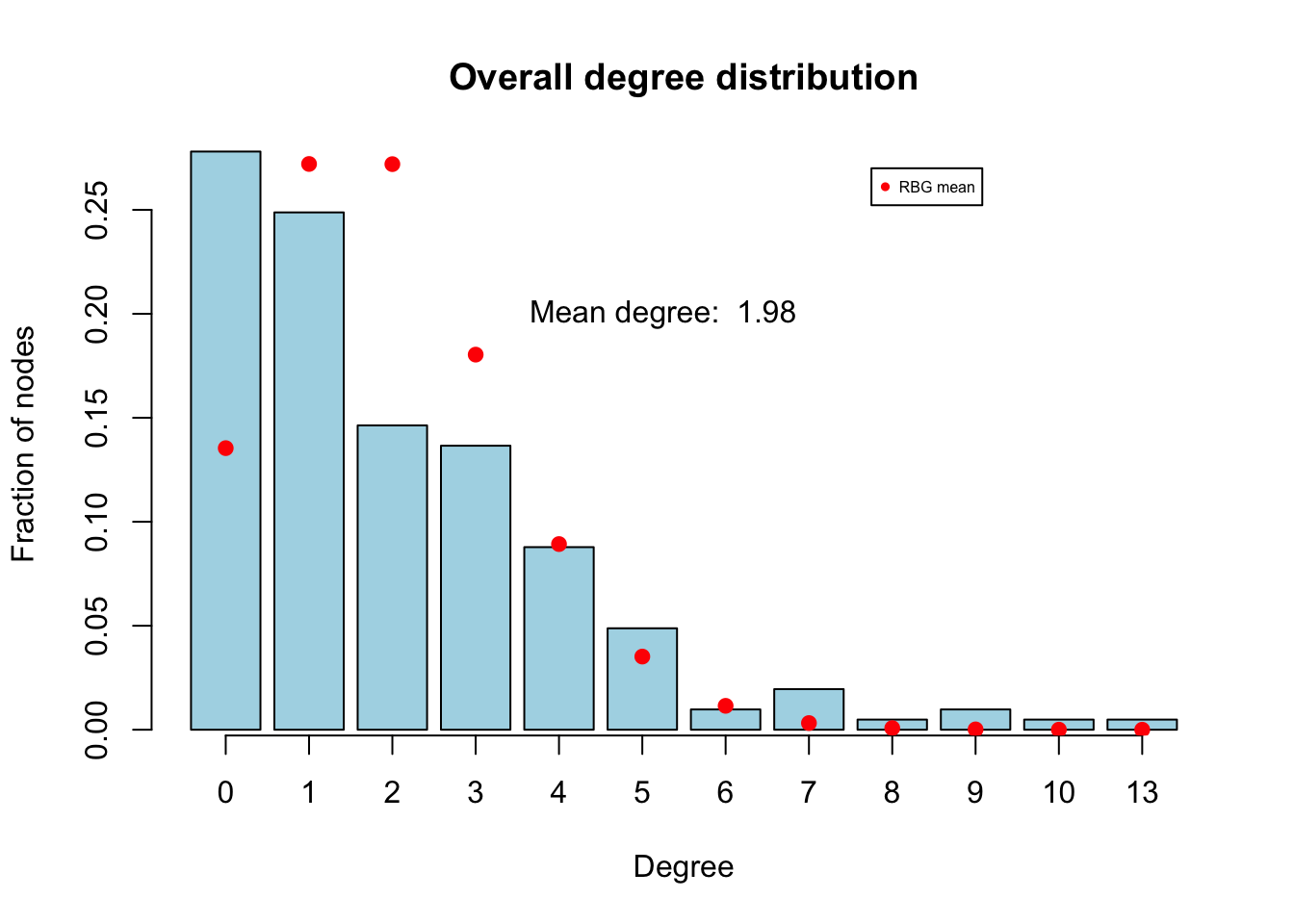
As we saw yesterday, the degree distribution shows large departures from the expected values given the mean degree in this network– particularly in the number of isolates.
When you see this kind of departure from expectation, this is your starting point for thinking about possible models. What kinds of network processes might account for the discrepancies you see here? Dyadic independent effects on tie formation (like nodal attribute-related differences)? Dyadic dependent effects on tie formation (like the degree and shared partner effects)?
It’s always worth starting with the dyad independent effects, and that’s what we will do here.
Heterogeneity in friendship activity levels by nodal attributes (like grade, race or sex) can potentially lead to patterns in the overall degree distribution that depart from the random graph expectations.
To get a quick descriptive read on whether this might be a productive direction for modeling we can plot the mean degree, broken down by nodal attributes. If there are visible differences we can capture these and test whether they are statistically significant in an ergm by using the nodefactor(attribute) terms.
Code
par(mfrow=c(1,2))
# by Grade
barplot(summary(mesa ~ nodefactor("Grade", levels=T)) / table(mesa %v% "Grade"),
horiz = T,
yaxt = "n", col = fill.col,
main = "Mean degree by Grade", xlab = "Mean degree", ylab = "Grade")
grades <- c(7:12)
pos <- barplot(summary(mesa ~ meandeg:nodefactor("Grade", levels=TRUE)),
horiz = T, plot=F)
axis(2, at = pos, labels = grades)
# by sex
barplot(summary(mesa ~ nodefactor("Sex", levels=T)) / table(mesa %v% "Sex"), horiz = T,
yaxt = "n", col=fill.col[7:8],
main = "Mean degree by Sex", xlab = "Mean degree", ylab = "Sex")
sex <- c("F", "M")
pos <- barplot(summary(mesa ~ meandeg:nodefactor("Sex", levels=TRUE)),
horiz = T, plot=F)
axis(2, at = pos, labels=sex)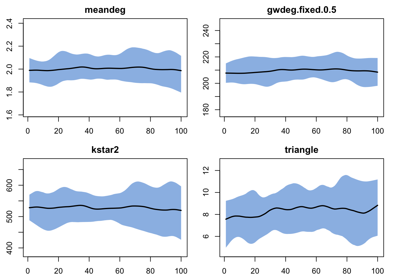
Statistical signicance is a test intended for inference from a sample to a population – it represents the effect of sampling variation on the uncertainty in an estimate. What does it mean to test for statistical significance when you have complete network data?
We can also consider whether the number of isolates – the biggest deviation we observed above in the degree distribution – varies by nodal attribute. Here we’ll just look at variation by sex.
Isolates by sex:
Another form of heterogeneity associated with nodal attributes is mixing patterns. The null hypothesis here is typically called “random” or “proportional” mixing, and implies that ties within and between group are formed in proportion to the group sizes (and potentially different contact rates). The general term for patterns that depart from proportional mixing is “selective” mixing.
There is a wide range of possible selective mixing patterns by attribute that one might observe. One of the most common patterns is “homophily”, also called “assortative” or “like-with-like” mixing. It is also possible to observe the opposite: disassortative mixing – the classic example of this is mixing by sex in a (mostly) heterosexual network. When the attribute is quantitative (like Grade) you might observe a smooth decline in ties as the quantitative difference in attributes increases. And in some cases the pattern may be idiosycratic, but still different than what one would expect under proportional mixing.
How you explore the patterns of attribute mixing in your data depends on the attribute metric (categorical, interval, continous). Here we have a categorical measure (Sex) and an interval level quantitative measure (Grade). Both have a limited number of categories, so they can be easily explored using mixing matrices – the cross-tabulation of ties by the attributes of each node – and network plots colored by attribute.
Note that because this is an undirected tie, and because we have the entire population represented, the mixing matrices must be symmetric. With sampled network data, you may see asymmetry in the number of ties reported.
- Mixing matrices
By Grade
7 8 9 10 11 12
7 75 0 0 1 1 1
8 0 33 2 4 2 1
9 0 2 23 7 6 4
10 1 4 7 9 1 5
11 1 2 6 1 17 5
12 1 1 4 5 5 6Note: Marginal totals can be misleading for undirected mixing matrices.By Sex
F M
F 82 71
M 71 50Note: Marginal totals can be misleading for undirected mixing matrices.It is possible to construct the expected values under the null hypothesis (can you think about what those calculations might look like?), but we won’t do that here. Instead, we will test for departures from the null using the nodematch(diff=T) term when we fit the ERGM.
- Network diagrams colored by Grade and Sex:
Code
par(mfrow = c(1,2), oma=c(0,0,3,0))
plot(mesa, coord=coords,
vertex.col='Grade', main="By Grade", cex.main = 1)
legend('bottomleft',fill=7:12,
legend=paste('Grade',7:12),cex=0.5)
plot(mesa, coord=coords,
vertex.col='Sex', main="By Sex", cex.main = 1)
legend('bottomleft',fill=1:2,
legend=paste('Sex',c("F","M")),cex=0.5)
mtext("Mesa friendship network", side=3, outer=T, cex=1.2)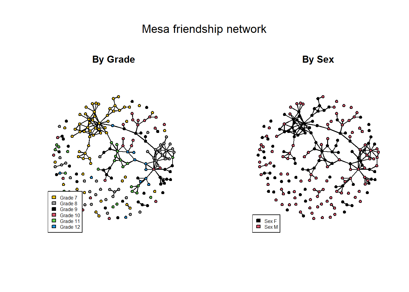
The EDA replicates what we saw in this network using statnetWeb yesterday: both the sex and grade attributes influence friendship prevalence and selection, producing a network with some clear heterogeneities in structure.
33.1.3 Specify the model
We explored several models in statnetWeb yesterday, but here we want to focus on demonstrating how network data are used in an EpiModel workflow. So we won’t spend time testing and comparing models for the network, but the lab will give you a chance to do some of that.
We are going to fit a specific model for attribute heterogeneities that is (loosely) informed by the EDA above:
- “main effects” for sex and grade (
nodefactor) – to capture the difference in mean degree by levels of each attribute; - a mixing term for grade (
nodematch) – to capture homophily by grade, here we assume an overall effect rather than grade-specific; - a mixing term for sex – to capture homophily by sex;
- a degree(0) term by sex – to capture the differential prevalence of isolates for boys and girls.
33.1.4 Fitting the Network Model
Following the terminology and syntax demonstrated previously, we would like to fit a TERGM where the formula includes terms for overall mean degree (edges), mean degree by grade and sex (nodefactor terms) mixing by grade (a nodematch term), and isolates by sex (having a degree of exactly zero). A total of 11 terms is specified by this model.
Since we are using network data input we can use ergm to calculate the summary statistics for these model terms directly from the data using the summary() function. These are the statistics used as the target stats in the fitting process.
Code
targets
edges 203
nodefactor.Grade.8 75
nodefactor.Grade.9 65
nodefactor.Grade.10 36
nodefactor.Grade.11 49
nodefactor.Grade.12 28
nodematch.Grade 163
nodefactor.Sex.M 171
nodematch.Sex 132
deg0.Sex.F 23
deg0.Sex.M 34To fit the TERGM, we will pass the formation formula and target stats from above, and a dissolution parameter. Since the Mesa data contain only information on the static network structure (which is summarized by our model target stats), we will specify the dissolution dynamics with a hypothetical value.
This is an example of the flexibility of EpiModel specification – you can work with observed data only, or mix observed and hypothetical inputs to explore their impacts.
We specify a hypothetical parameter for the dissolution model that produces a mean relational duration of 60 time steps.
Note, you can modify this and see how it influences the fit and the network dynamics.
Code
Call:
ergm(formula = formation, constraints = constraints, offset.coef = coef.form,
target.stats = target.stats, eval.loglik = FALSE, control = set.control.ergm,
verbose = verbose, basis = nw)
Monte Carlo Maximum Likelihood Results:
Estimate Std. Error MCMC % z value Pr(>|z|)
edges -6.12316 0.23287 0 -26.294 < 1e-04 ***
nodefactor.Grade.8 0.19752 0.07504 0 2.632 0.008486 **
nodefactor.Grade.9 0.09021 0.07176 0 1.257 0.208709
nodefactor.Grade.10 0.33930 0.09610 0 3.531 0.000414 ***
nodefactor.Grade.11 0.45217 0.08964 0 5.044 < 1e-04 ***
nodefactor.Grade.12 0.77903 0.12666 0 6.151 < 1e-04 ***
nodematch.Grade 3.00502 0.17869 0 16.817 < 1e-04 ***
nodefactor.Sex.M -0.27472 0.11356 0 -2.419 0.015561 *
nodematch.Sex 0.60926 0.14794 0 4.118 < 1e-04 ***
deg0.Sex.F 1.66104 0.31293 0 5.308 < 1e-04 ***
deg0.Sex.M 1.21999 0.30441 0 4.008 < 1e-04 ***
---
Signif. codes: 0 '***' 0.001 '**' 0.01 '*' 0.05 '.' 0.1 ' ' 1
Dissolution Coefficients
=======================
Dissolution Model: ~offset(edges)
Target Statistics: 60
Crude Coefficient: 4.077537
Mortality/Exit Rate: 0
Adjusted Coefficient: 4.077537Let’s take a moment to look at the coefficients, and think about how these summarize the way the friendship tie patterns depart from a simple BRG.
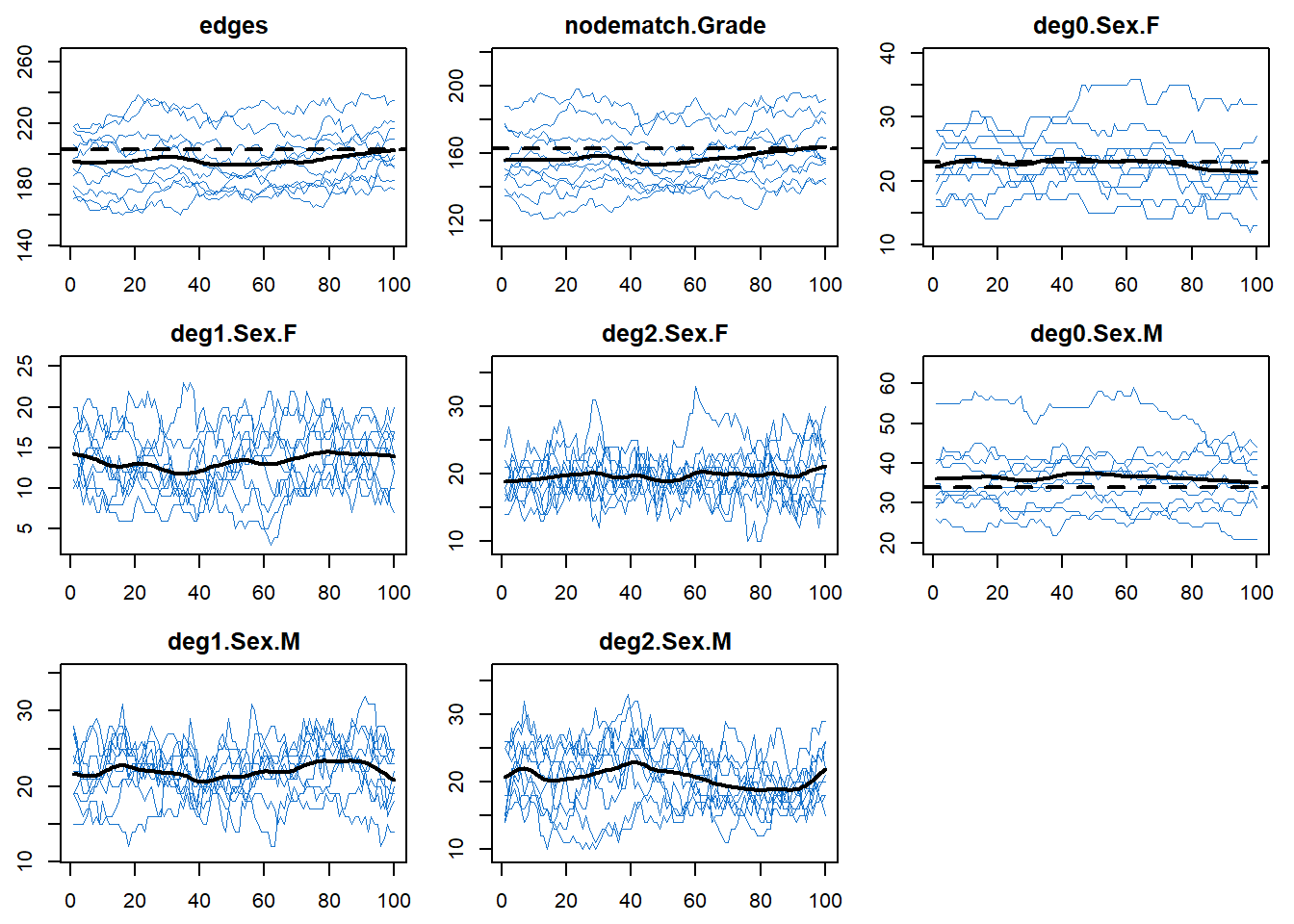
33.1.5 Diagnose the model fit
33.1.5.1 Convergence assessment
First, we run convergence diagnostics to verify that the target stats are reproduced in expectation. If they are not, we would need to go back to the fit call and address the problem there. There are many fit diagnostics tuning parameters in ergm/tergm for improving model convergence. We will not need those here, but it is important to know about them if your target stat diagnostic plots show problems.
33.1.5.2 GOF validation
And as we showed yesterday, we can also run dx for network statistics we did not include in the model.
This is a form of model validation – to assess how well the model reproduces network features that were excluded.
To run the default GOF stats – the full degree, esp and geodesic distributions – we need to extract the fit object from the output object produced by netest and use ergm functionality directly on that fit object, since EpiModel does not have a dedicated command for the default GOF plots.
[1] "formation" "target.stats" "target.stats.names"
[4] "coef.form" "coef.form.crude" "coef.diss"
[7] "constraints" "edapprox" "nested.edapprox"
[10] "newnetwork" "formula" "summary"
[13] "fit" Sampling ■■■■■■■■■■■ 35% | ETA: 5sSampling ■■■■■■■■■■■■■■■■■■■■■■■■ 77% | ETA: 2s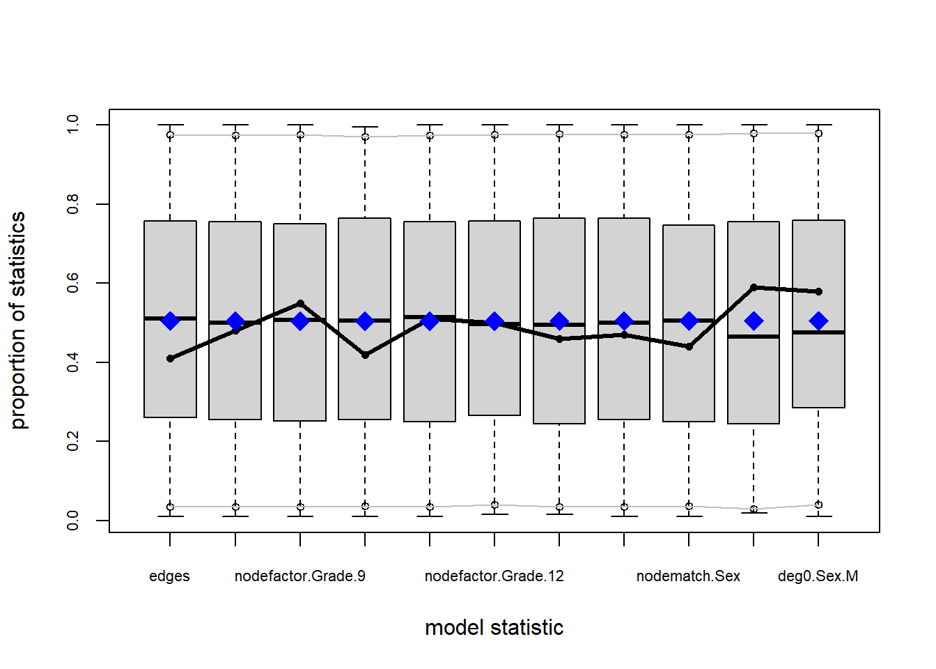
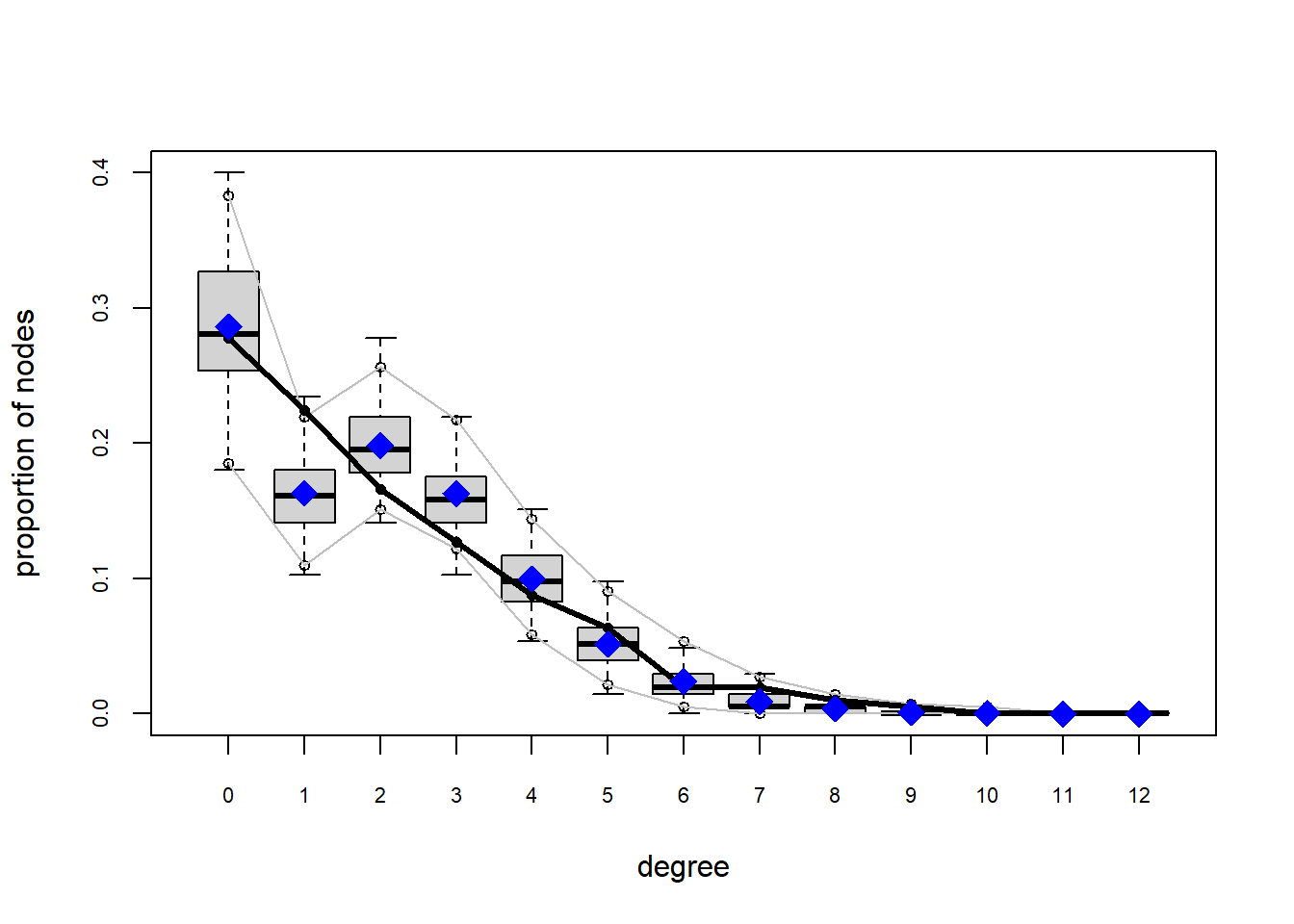
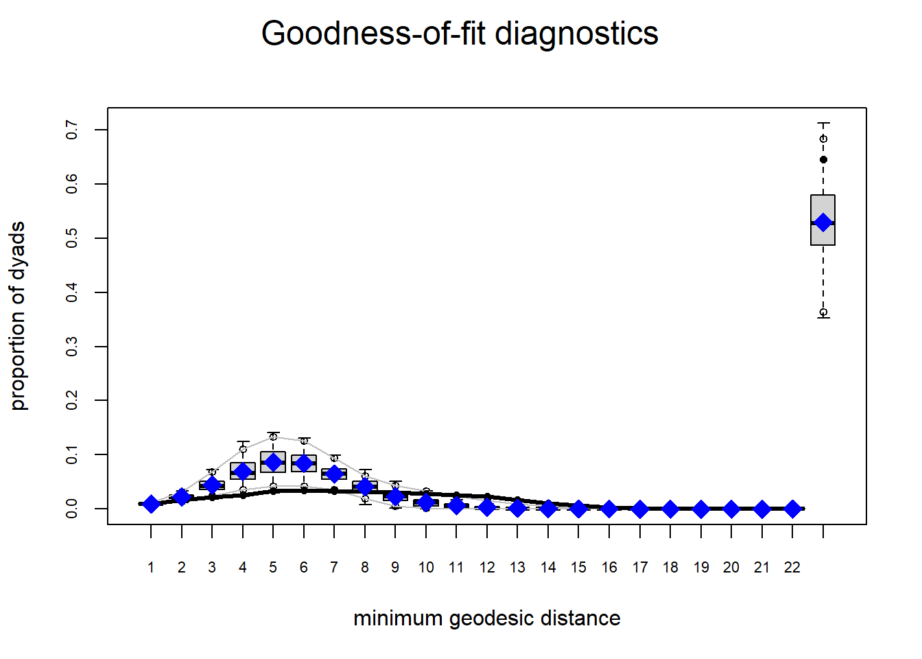
So we see a pattern that looks similar to the models we assessed yesterday:
We can fit the degree 0 deviation by including deg0 terms in the model (here we did it allowing for heterogeity by sex), but we still don’t get the rest of the degree distribution right when we do that.
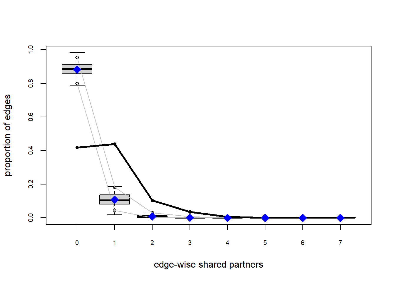
This model does not reproduce the observed ESP distribution (not even close)
It also doesn’t do a good job on the geodesic distribution.
We are not restricted to the default GOF validation statistics, we can consider any observable netstats.
So let’s take a look at some different statistics:
obs
 meandeg
1.980488
gwdeg.fixed.0.5 199.565738
kstar2 659.000000
triangle 62.000000Note that two of the problematic “Markov terms” we identified yesterday are included in this summary call: kstar and triangles. They don’t cause a problem here because we are just counting their prevalence in the network, not estimating parameters for a model with these terms.
Let’s compare these observed values to the stats produced by this fitted model.
Code
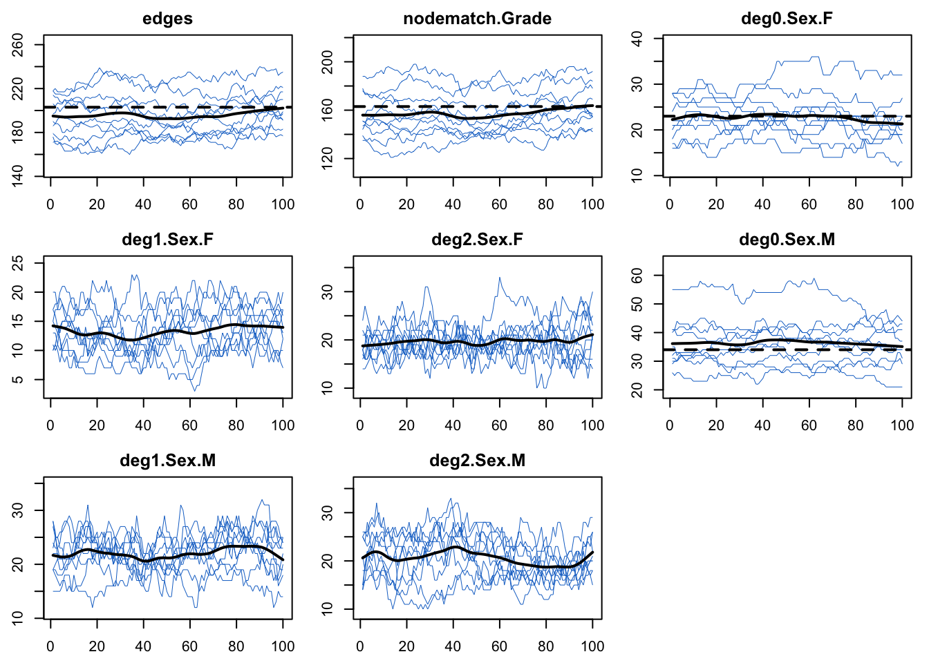
Network Diagnostics
-----------------------
- Simulating 25 networks
- Calculating formation statistics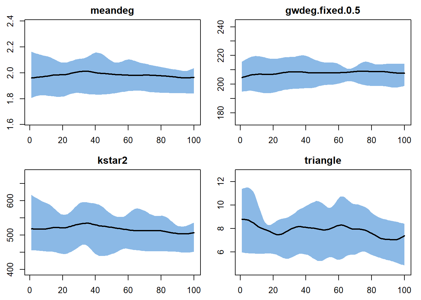
Which of the excluded netstats are reproduced by the model? Which are not?
One could do much more work on model specification here, but we will move on to simulating an epidemic across this network. Keeping in mind:
The network structure in our simulated networks WILL reproduce the network statistics in the model: the nodefactor, nodematch and degree 0 stats.
But they will not reproduce ALL of the patterns we observe in our network. In particular we are still getting the local clustering (ESP, kstar, triangle) right, and are also not fitting the geodesics perfectly.
33.1.6 Epidemic Simulation
To run an epidemic process over a dynamic network simulated from this model fit, we need to set up the epidemic model parameters, initial conditions, and control settings (you can review the details in this chapter). In this example, we will specify values for a hypothetical infection.
Code
myparam <- param.net(inf.prob = 0.2,
act.rate = 1.8,
rec.rate = 0.1)
myinit <- init.net(i.num = 10)
# Here we set which attribute to use for epi stats breakdowns with "epi.by"
# (only one can be specified in base EpiModel)
# and also which stats we want to monitor with "nwstats.formula"
mycontrol <- control.net("SIS", nsteps = 100, nsims = 10,
epi.by = "Grade",
nwstats.formula = ~edges + nodematch("Grade") +
degree(0:2, by = "Sex"),
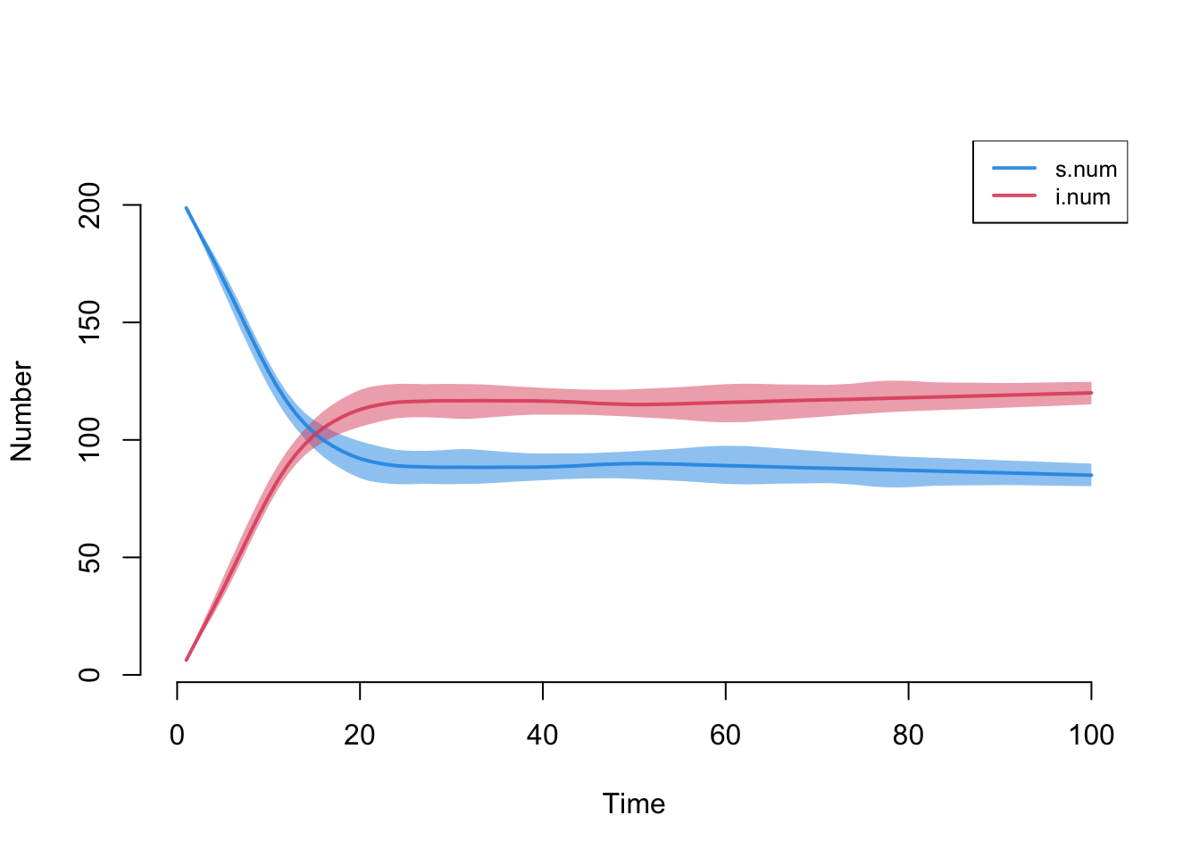
verbose = TRUE)Now we can run the epidemic simulation with netsim. The prevalence rate trajectory is plotted below. With this simple SIS model, and starting with about 5% of the population infected (i.num = 10, population size = 205), the epidemic reaches equilibrium pretty quickly.
Does the equilibrium prevalence surprise you? Why or why not?
Code
The ERGM fit showed pretty large differences in mean degree by grade, as well as a strong propensity for within grade mixing.
Would you expect prevalence to vary by grade?
Since the grade sizes are unequal, it’s best to compare rates rather than raw numbers. We construct and plot those below.
Code
mySIS <- mutate_epi(mySIS,
                    prev.7 = i.num.Grade7 / num.Grade7,
                    prev.8 = i.num.Grade8 / num.Grade8,
                    prev.9 = i.num.Grade9 / num.Grade9,
                    prev.10 = i.num.Grade10 / num.Grade10,
                    prev.11 = i.num.Grade11 / num.Grade11,
                    prev.12 = i.num.Grade12 / num.Grade12)

plot(mySIS, y = c("prev.7", "prev.8", "prev.9", "prev.10",
                  "prev.11", "prev.12"),
     ylab = "Prevalence",
     qnts.alpha = 0.2, qnts = 0.5, legend = TRUE)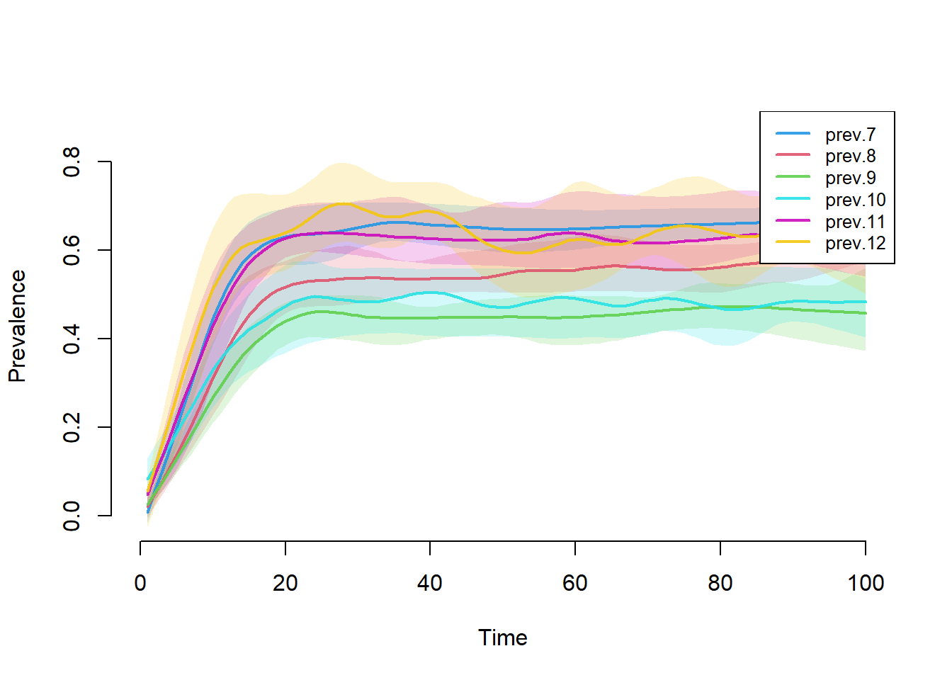
There are some prevalence differentials at equilibrium – lower prevalence for the 8/9/10th graders, and higher for the 7/11/12th graders – and these correspond to the mean degree differentials we see in the ERGM coefficients.
The prevalence stabilizes at a range of roughly 45-60% for all grades, so the equilibrium rate of infection is fairly high for all Grades, despite the differentials. This happens because the transmission probability is relatively high, the network is relatively well connected over time and there are no groups that are completely isolated from the others.
It’s also a good idea to plot the modeled network stats time series from the epidemic simulations to ensure that the epidemic simulations did not have unintended consequences on the network structure. Here, because we are working with a closed population (no births or deaths) and we did not model any behavior changes associated with infection, the network should not change once the epidemic is introduced, it should remain (stochastically) stable. So if we see large deviations from the targets, that would suggest an error in the coding somewhere.
33.1.7 Dynamic Visualization
The simulation object you created can be passed to the ndtv package for animation, allowing you to see how the infection moves through the network of students. Recall that the while the network data we started with is a network census, it is a static network. So we passed a hyptothetical average partnership duration to EpiModel for calculating the dissolution model and parameterizing the TERGM. That means the network structure is coming from the observed data, and the dynamics of tie formation and dissolution from the hypothetical.
We’ll vizualize the first 20 steps of the epidemic simulation to get a sense of what the network, and the spread, look like.
Code
myEpiSim <- get_network(mySIS)
myEpiSim <- color_tea(myEpiSim, verbose = FALSE)

slice.par <- list(start = 1, end = 20, interval = 1,
                  aggregate.dur = 1, rule = "any")
render.par <- list(tween.frames = 10, show.time = FALSE)
plot.par <- list(mar = c(0, 0, 0, 0))

compute.animation(myEpiSim, slice.par = slice.par, verbose = TRUE)
render.d3movie(
  myEpiSim,
  render.par = render.par,
  plot.par = plot.par,
  vertex.cex = 0.9,
  vertex.col = "ndtvcol",
  edge.col = "darkgrey",
  vertex.border = "lightgrey",
  displaylabels = FALSE,
  output.mode = "htmlWidget")
Given what you know about this network, how well do you think this simulated model captures the heterogeneity in friendship structure? Does the animated network seem to have the same structure as the observed network over time? If not, how would you modify the workflow above to address this?
So that’s the workflow when working with a network census dataset and a hypothetical edge duration parameter. Behind the curtain, this is the breakdown of how the packages are used:
netest()
the
ergmpackage calculates the target statistics from the network data and estimates the formation model that you specified for the faux.mesa.high nodeset.the
EpiModelpackage calculates the dissolution coefficient and adjusts the coefficient on theedgesterm of the formation model to transform it to an incidence rate.
netdx()
- the
tergmpackage simulates a complete dynamic network over time from the fitted model and keeps a list of the monitored statistics for inspection/plotting
netsim()
the
tergmpackage simulates a complete dynamic network over time from the fitted model (as above).the
EpiModelpackage simulates the transmission process over the dynamic network
- animation
EpiModelextracts the network and colors the nodes by infection status (get_network,color_tea)ndtvanimates the colored dynamic network (withcompute.animationandrender.d3movie)
33.2 Egocentric network data
Now we will extract the ego networks from Mesa, fit the same network model, and run the same epidemic simulation. The only difference is that we are now using an egocentric view of the data, and passing this as the input for EpiModel (and, behind the scenes, ergm and tergm).
It’s worth noting what is the same, and what is different in this (very) artificial example.
- What is the same: we have exactly the same nodes with exactly the same attributes in both the network census and the egocentric census of the network.
Having the same number of nodes in and egocentric sample as in the population is not realistic – you would almost never set out to conduct an egocentric “census” study design. The whole point of egocentric network sampling is to reduce the burden of data collection while leveraging the principles of statistics for inference to the population network.
But it is intentional here. The primary goal of this tutorial is to show that you get the same analytic results (from the statnet and EpiModel tools), from both data types, when they contain the same information. That is the best way to demonstrate that egocentric data inputs produce valid and reliable results.
- What is different: In the egocentric sample, the alters are not uniquely “identifiable”. The alter attributes are observed (Grade, Race, Sex), but not their unique id. We also do not make use of the “alter-alter” matrix (though this is extracted from Mesa when we transform it to an egocentric view object, we will ignore it).
Effectively, this limits what we “see” in the egocentric dataset to ego degree, the heterogeneities in that degree, and mixing by attributes that are recorded for both ego and alter. Because of that, there are many network statistics we can no longer observe: no edgewise shared partners, no triangles, no geodesics.
The primary limitation this imposes is on the network statistics that can be used in a model or in a validation GOF (to test for excluded netstats).
But this limitation does not extend to networks we simulate from the fitted model, and in these simulated networks, all of the network statistics are again visible. Through simulation we can sample from the space of networks defined by the model: the realizations are (stochastically) constrained to have the same sufficient statistics as our observed egocentric data. This gives us a powerful tool for making further inferences.
- For example, we can simulate 10,000 networks from the model and calculate the geodesic distribution from each. From this we can see how much variation there is in the mean geodesic (or in any other property of the geodesic distribution, like the range, or the IQR). If there is little variation in the mean geodesic (or another summary geodesic stat), that suggests the statistics in our model terms constrain the behavior of this this global network property, and we can predict what it is likely to be, even though we haven’t observed in in our egocentric data. If, on the other hand, there is a lot of variation in the simulated mean geodesics, then we know our model terms are consistent with many different global network structures, and we have a limited ability to predict the value in the true population network from the egocentric data.
As long as our egos are a representative sample from the population, we can make inferences from the properties we observe in simulated networks sampled from the fitted model to the population, and assess their uncertainty.
33.2.1 Load the ergm.ego package
The ergm.ego package is designed to fit ERGMs to egocentrically sampled network data. There are many differences in the analytic process for egocentrically sampled data, from data storage structures and manipulation to estimation and inference.
While we have discussed the basic statistical principles that support using sufficient statistics to estimate an ERGM, we have not gone into the details of implementing this for an egocentric data source. Briefly, it is a two step process: the first step scales the network statistics to a self-weighted population of nodes, the second estimates the ERGM on a complete network with the self-weighted nodeset, using the scaled sufficient statistics.
More details on the statistical framework for estimation and inference can be found in the Appendix to this module, and relies on the paper by Krivitsky and Morris, 2017.
For more practical discussion of the software utilities in ergm.ego, please see ?ergm.ego and the Statnet ergm.ego workshop.
Here, we will give a brief overview of the data storage object used in ergm.ego – an egor object – demonstrate a few of the utilities in the package, and show how to use egocentric data as an input to the EpiModel package, replicating the full workflow.
33.2.2 Extract the egocentric data
We start by extracting an egocentric census from the Mesa network – that is, we pull the egonets for every node in the network.
The object we extract from Mesa is an egor class object (egor is also the name of the package that handles egodata), and it’s a list that contains 3 tables:
egos (with their attributes),
alters (with their attributes and the egoID they are linked to) and
aaties (if these are present).
The format of the summary information is different than the format used with network objects. For more details about the structure of egor objects and how to work with them please see ?as.egor and the Statnet ergm.ego workshop.
[1] "egor" "list"# EGO data (active): 205 × 4
.egoID Grade Race Sex
* <int> <dbl> <chr> <chr>
1 1 7 Hisp F
2 2 7 Hisp F
3 3 11 NatAm M
4 4 8 Hisp M
5 5 10 White F
# ℹ 200 more rows
# ALTER data: 406 × 5
.altID .egoID Grade Race Sex
* <int> <int> <dbl> <chr> <chr>
1 174 1 7 Hisp F
2 161 1 7 Hisp F
3 151 1 7 Hisp F
# ℹ 403 more rows
# AATIE data: 372 × 3
.egoID .srcID .tgtID
* <int> <int> <int>
1 1 151 127
2 1 127 52
3 1 127 87
# ℹ 369 more rows205 Egos/ Ego Networks
406 Alters
Min. Netsize 0
Average Netsize 1.98048780487805
Max. Netsize 13
Average Density 0.750903163274297
Alter survey design:
Maximum nominations: Inf Let’s verify that the ego attribute distribution is the same as in the Mesa network object.
- The distributions
      F  M
  7  35 27
  8  15 25
  9  22 20
  10 10 15
  11 10 14
  12  7  5
      F  M
  7  35 27
  8  15 25
  9  22 20
  10 10 15
  11 10 14
12 7 5- The difference
33.2.3 Explore the data
The simple structure of the egor object makes it relatively easy to conduct EDA using the traditional tools in R, and examples can be found in the Statnet workshop for ergm-ego.
ergm.egohas utilities for working with survey weights and design specifications (if your data has these).
This information must be added to the egor object using the ego_design function. Once you add a design, the structure of the egor object changes, and the designed element (typically the egos) becomes an srvyr object. When you calculate summary statistics or estimate an ERGM with the object it will automatically include the weights appropriately in the analysis. We will not demo all of that functionality in this tutorial, but it is worth knowing that it is there.
We’ll just highlight one nice plotting function built into ergm-ego for looking at degree distributions by attributes, with the BRG distribution overlay. Note this is the same type of plot you saw using statnetWeb, but now we can add a breakdown by attribute.
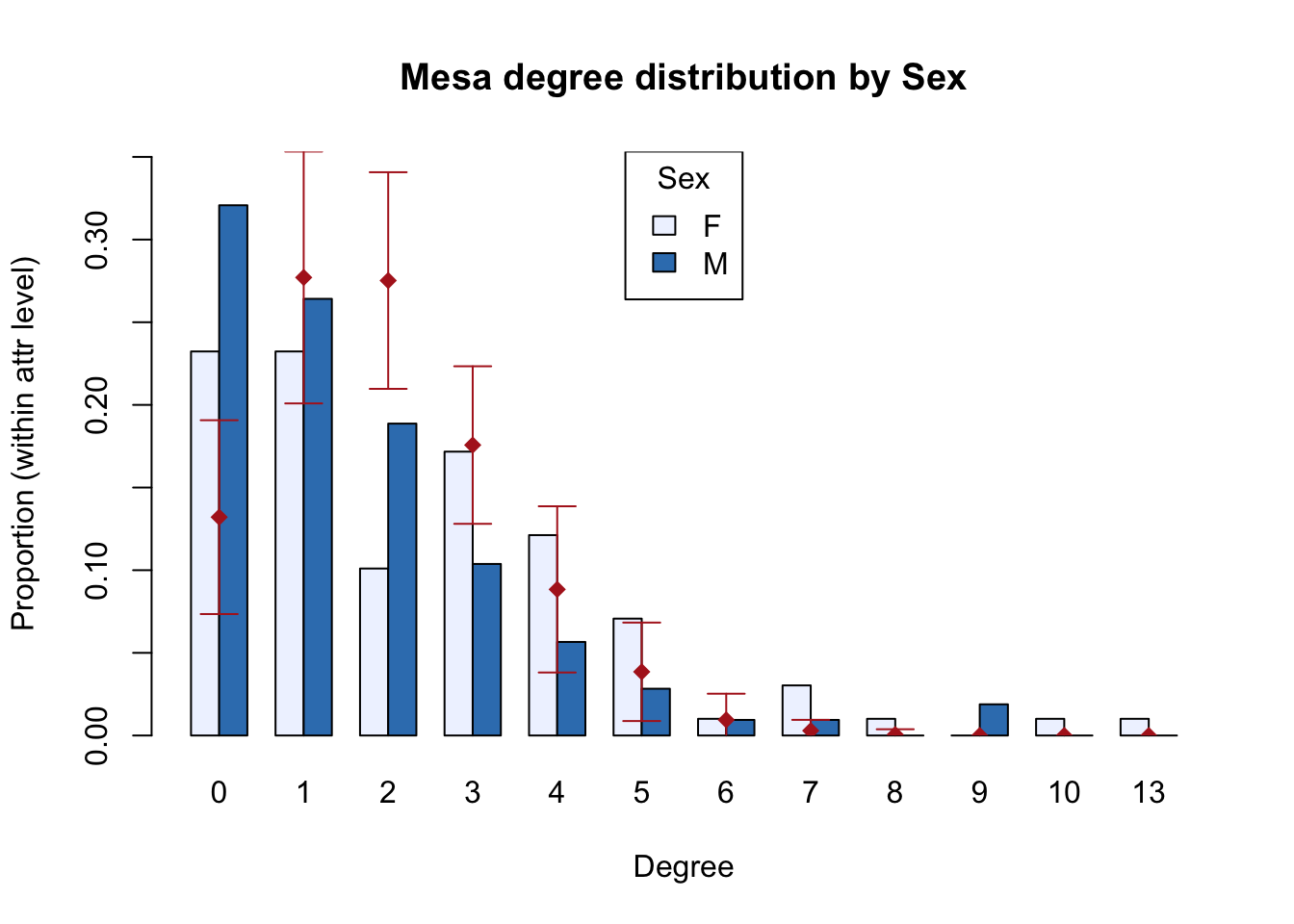

Let’s look at one other important thing: the summary statistics for the model terms from the two types of network data. These stats become the target stats in the fitting process.
Code
                    network egocensus
edges                   203       203
nodefactor.Grade.8       75        75
nodefactor.Grade.9       65        65
nodefactor.Grade.10      36        36
nodefactor.Grade.11      49        49
nodefactor.Grade.12      28        28
nodematch.Grade         163       163
nodefactor.Sex.M        171       171
nodematch.Sex           132       132
deg0.Sex.F               23        23
deg0.Sex.M               34        34
They’re identical. So, net of stochastic variation in the fitting algorithm, the ERGM and STERGM fits from these two different network data inputs should be the same.
33.2.4 Fit the network model
We fit the STERGM using netest with the same formula we used for the network census. This time, netest will automatically detect that the network object passed on the LHS is an egor object, and it will use ergm.ego for the estimation.
When fit without specific population size controls, the
ergm.egopackage default assumption is that the desired network size is equal to the sample size.
We’ll use this default here, since we took a census of our true population network, Mesa, so our egocentric “sample” actually is the same size as our population network. But we’ll show an example of scaling the fit to a different population network size below.
Compare the coefficients from the two fits (the same, net of stochastic variations in the fitting algorithm):
Code
                    network egocensus   diff
edges                -6.123    -6.129  0.006
nodefactor.Grade.8    0.198     0.187  0.010
nodefactor.Grade.9    0.090     0.094 -0.004
nodefactor.Grade.10   0.339     0.337  0.002
nodefactor.Grade.11   0.452     0.454 -0.002
nodefactor.Grade.12   0.779     0.768  0.011
nodematch.Grade       3.005     3.005  0.000
nodefactor.Sex.M     -0.275    -0.275  0.001
nodematch.Sex         0.609     0.619 -0.010
deg0.Sex.F            1.661     1.661  0.000
deg0.Sex.M            1.220     1.216  0.004
Run model diagnostics to check the model goodness of fit with the egodata and plot the results:
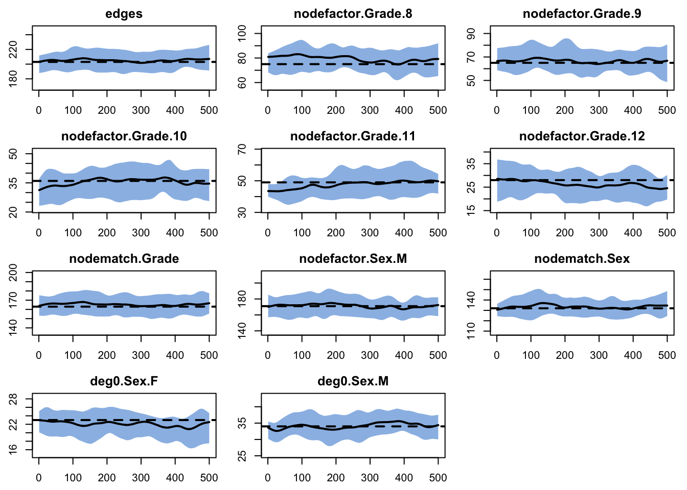
As with the network census data, the simulations from the egodata census match the target statistics in expectation.
We won’t go on to simulate the epidemic, since the inputs to and syntax for EpiModel from here forward are the same as those used for the Mesa network census above.
But note that following that workflow, what you get at the end is a simulated complete dynamic network, with an epidemic and a movie. All from the minimal data of a cross-sectional representative egocentric sample + average tie duration.
Bottom line: The basic netest syntax is similar for all types of network data inputs – target statistics, a network census dataset or egocentrically sampled network data.
Since ERGM/TERGM fits depend only on the model’s sufficient statistics, when the values of these statistics are the same, the estimated coefficients, network simulations and epidemic simulations will be the same (up to stochastic variation), regardless of the type of data that you pass to EpiModel.
33.2.5 Scale the fit to a different network size
ergm.ego estimation is performed by constructing a complete network “pseudo-population” with appropriately scaled sufficient statistics. You can modify the size of this “pseudo-population”, which will then estimate the model for a larger (or smaller) network. This is useful in several contexts:
Your egocentrically sampled dataset has weights.
Egocentric study designs are used just like a sample survey: to collect data from a tiny fraction of the whole population, and use the sample to estimate models and make statistical inferences to the whole population. Sampling is efficient (when it’s done right!), and most efficient sampling uses stratification weights. When your sample has weights,
ergm.egoestimation is performed on a self-weighted complete pseudo-network – that is, a pseudo-population of nodes with the composition implied by the sample weights. When scaling the nodeset to have the right composition a simple rule of thumb is that the node with the smallest weight should be represented at least once, though more is better.Your egocentrically sampled dataset is small.
Statistical studies performed in Krivitsky and Morris, 2017 suggest a good rule of thumb to minimize bias is to estimate with a minimum “pseudo-population” network size of 1,000 when using unweighted data. But note the appropriate size depends on the complexity of the model, as in other statistical contexts.
Simulation experiments (“what-ifs” and counterfactuals)
Say you want to examine whether and how network size influences infection dynamics. One way to do that is to fit the network model with a range of explicit pseudo-population sizes, simulate epidemics on these differently sized networks, and compare the results.
It is helpful to learn a bit more about how the package ergm.ego works if you want to explore model-based network scaling, but the basic netest syntax itself is very simple – you pass the argument ppopsize to ergm.ego via the argument set.control.ergm.ego in netest. Here we demonstrate estimation with pseudo-population network sizes of 1000 and 2000.
Code
set.seed(0)
myfit.ego.pp1000 <- netest(mesa.ego,
                           formation = formation,
                           coef.diss = dissolution_coefs(~offset(edges), 60),
                           set.control.ergm.ego = ergm.ego::control.ergm.ego(
                             ppopsize = 1000))

set.seed(0)
myfit.ego.pp2000 <- netest(mesa.ego,
                           formation = formation,
                           coef.diss = dissolution_coefs(~offset(edges), 60),
                           set.control.ergm.ego = ergm.ego::control.ergm.ego(
                             ppopsize = 2000))
The control parameter tells ergm.ego to construct a complete network of size ppopsize with the same (proportional) distribution of nodal attributes, same mean degree and appropriately scaled target statistics as those observed in the egocentric sample (or as close as possible if the ppopsize is not a multiple of the sample size). The MCMC fitting algorithm then uses this scaled pseudo-network during estimation.
If you want to inspect the scaled pseudo-network, it can be found in the fit object component newnetwork. This is technically the network used in the last chain of the MCMC estimation process, so the ties are a stochastic draw from the model distribution, but the target stats and nodeset (with attributes) are the same throughout the fitting process.
Compare the number of nodes in each of the networks, their target stats, and the preservation of mean degree across network size (net of stochasticity):
- Network sizes
Code
  network egocensus egopp1000 egopp2000
1 205 205 1025 2050- Scaling factor for network size
Code
  network egocensus egopp1000 egopp2000
1 1 1 5 10- Target stats
Target stats: Code
                    network egocensus egopp1000 egopp2000
edges                   203       203      1015      2030
nodefactor.Grade.8       75        75       375       750
nodefactor.Grade.9       65        65       325       650
nodefactor.Grade.10      36        36       180       360
nodefactor.Grade.11      49        49       245       490
nodefactor.Grade.12      28        28       140       280
nodematch.Grade         163       163       815      1630
nodefactor.Sex.M        171       171       855      1710
nodematch.Sex           132       132       660      1320
deg0.Sex.F               23        23       115       230
deg0.Sex.M 34 34 170 340- Scaling factor for target stats
Code
                    network egocensus egopp1000 egopp2000
edges                     1         1         5        10
nodefactor.Grade.8        1         1         5        10
nodefactor.Grade.9        1         1         5        10
nodefactor.Grade.10       1         1         5        10
nodefactor.Grade.11       1         1         5        10
nodefactor.Grade.12       1         1         5        10
nodematch.Grade           1         1         5        10
nodefactor.Sex.M          1         1         5        10
nodematch.Sex             1         1         5        10
deg0.Sex.F                1         1         5        10
deg0.Sex.M 1 1 5 10- Mean degree (in the final network from the MCMC chain)
Code
        network egocensus egopp1000 egopp2000
meandeg 2.17561 2.234146 1.976585 2.044878- Estimated network model coefficients:
Code
                    network egocensus egopp1000 egopp2000 pct.diff2000
edges                -6.123    -6.129    -7.669    -8.356      -36.467
nodefactor.Grade.8    0.198     0.187     0.175     0.173       12.650
nodefactor.Grade.9    0.090     0.094     0.079     0.078       14.057
nodefactor.Grade.10   0.339     0.337     0.305     0.304       10.454
nodefactor.Grade.11   0.452     0.454     0.410     0.407        9.979
nodefactor.Grade.12   0.779     0.768     0.697     0.683       12.264
nodematch.Grade       3.005     3.005     2.898     2.889        3.877
nodefactor.Sex.M     -0.275    -0.275    -0.261    -0.260        5.235
nodematch.Sex         0.609     0.619     0.558     0.547       10.263
deg0.Sex.F            1.661     1.661     1.594     1.584        4.666
deg0.Sex.M            1.220     1.216     1.168     1.156        5.224
The key difference is the value of the “edges” coefficient, reflecting a scaling assumption built in to the ergm-ego package.
33.2.5.1 The scaling assumption: mean degree? or density?
The canonical edges coefficient in an ERGM controls the density of the network: the probability of a tie across all possible dyads. Recall that density is related to mean degree as:
\[ Mean Degree = Density * (N-1) \] We can verify this in the original Mesa network, by taking the ratio of mean degree to density:
Code
[1] 204As we scale up the network size, \(N' = k*N\), where \(k\) is 5 and 10 in our scaleup examples above, the number of dyads grows (as the square of the net size). If we use the fitted ERGM from the original Mesa network to simulate a network that is 5 or 10 times higher, the canonical edges coefficient would preserve the network density, but that would force the mean degree to rise, by a factor of \((k-1)*Density\). Using the Mesa network, for example, the mean degree would rise from the observed value of about 2 to about 8 and 20 respectively for our 1000 and 2000 sized networks.
This “density-dependent” behavior does not seem realistic in the context of most human social networks. Instead, it seems more likely that the number of ties a person has are likely to level out at a certain number, regardless of how much the population size increases (or decreases, as long as network size doesn’t drop below mean degree).
The ergm-ego package has a built-in assumption that preserves the mean degree rather than the density when network size is scaled up using the ppopsize argument.
Mean degree is preserved by the scaling the edges coefficient. The adjustment happens automatically in ergm.ego and is a straightforward difference on the log scale: log(orig net size) - log(new net size).
Note that the same assumption, that mean degree is the scale invariant parameter, is used in the EpiModel package, and is invoked when using open-population models.