54 Appendix: Improving Model Estimation and Simulation

54.1 Introduction

In this unit we dive deeper into the processes of estimation (a.k.a. “fitting”) and simulation for our network models, covering some of the common issues that users may face along the way. Typically, these will emerge as users explore one or more of the following relative to the examples we begin with in our tutorials:

more complex network models
sparser network models (those with lower overall relational density)
models on larger populations
models with shorter relational durations

We cover how to diagnose what is happening, and common approaches to fine-tuning the underlying algorithms to obtain convergence and desired behavior.

Two scoping notes before we start. First, the later sections are a reference rather than a course in ERGM/TERGM estimation. For the underlying algorithms (MCMLE, SAN, MCMC sampling), see the ergm and tergm papers (Krivitsky et al. 2023; Krivitsky and Handcock 2014) and the statnet workshops. Second, one whole class of fitting failures is not a controls problem at all: when relational durations are short or density is high, the edges-dissolution approximation (edapprox = TRUE) is itself insufficient and no amount of tuning rescues it. That boundary is what the full TERGM sections below are for.

After some initial setup, we proceed in the order:

Refresher on default model estimation in netest
Conducting full tergm estimation (i.e. when edapprox = FALSE)
Fine-tuning ergm estimation (i.e. when edapprox = TRUE)
Fine-tuning simulation (including diagnostics)

The controls themselves live at two stages, and a fit that misbehaves is almost always fixed at one of them. Estimation controls (control.ergm, passed to netest() via set.control.ergm) govern how the cross-sectional model is fit. Simulation controls (control.simulate.formula.tergm, passed to netdx() and netsim() via set.control.tergm) govern how the fitted model is stepped forward, both in diagnostics and in the epidemic run. Knowing which stage you are debugging is most of the work.

We then close with the applied material: two diagnosis traps that commonly waste time, a worked case of a fit that stalled for a day, and two practical shortcuts.

Remember that you learned about the basic set of steps in model estimation here. Specifically, the basic algorithm used during ergm estimation is:

Specify a model and calculate the sufficient statistics $g(y)$
Set a starting value for your vector of coefficients, $\theta$
Simulate networks from a model with this $\theta$ vector
- Select a dyad at random (possibly with weights)
- Propose a tie between the 2 nodes: “toggle”
  - Some are accepted, some not, based on the probability defined by this $\theta$ vector
- Every X toggles, grab the network and calculate the stats $g(y_{sim(i)})$
- Repeat this step Y times
After Y sampled networks:
- Compare the mean of $g(y_{sim})$ sample to the target stats $g(y)$
- Adjust the coefficients as indicated by the difference (higher or lower)
Repeat steps 3 & 4 until $g(y_{sim})$ converges to $g(y)$ and the sampling uncertainty is low

That covers the basics of estimation for ERGMs; note that it contains a loop within a loop, which makes it time-consuming and memory intensive. And the larger the network, or the more complex the model, the higher that X and Y typically need to be.

Extending this to TERGMs means adding an entire additional layer of looping: one must perform the above algorithm enough times within a single time step to reach the amount of change expected between two consecutive time steps just to get one sample, then repeat over and over for multiple time steps. This increases the computing time and complexity in parallel.

A few things to note before we get started:

This material (developed July 2026) still only scratches the surface. We aim to continue building out our guidance here, in multiple forms, including a longer tutorial, a vignette, and/or an EpiModel gallery example. Stay tuned!
We will walk through a few examples here, and then present tables of additional function arguments that one may use beyond those explored here. It is worth working through the examples at least once rather than just jumping straight to the tables, as they help give a feel for how these play out in practice. After that, the tables should serve as useful references to return to as needed.
One can make some progress in diagnosing and fitting models with only a passing understanding of the algorithms that are involved. For some users, that may be enough to get where they need to go on their research models. For more and more complex models, however, a greater familiarity with the algorithms becomes increasingly important. We aim to stay as high-level as possible on the algorithms here, and point users to more advanced material at the end if needed.
Setting the fitting parameters is often an iterative process. Set them too low, and the algorithm might fail. Set them too high, and the algorithm might take many hours (or even days!) longer than needed. The latter might seem preferable in most circumstances, but if one is expecting to estimate many similar models, then there is added incentive to find a reasonably efficient set of fitting parameter values that lead to success.
You may receive error messages during this estimation process, even though the estimation process continues. One common example is Error in xTAx_eigen(x, A, tol = tol, ...). These come from functions multiple layers down from netest in the function call stack. As long as the estimation process keeps running, you can assume that the algorithm has some means of adjusting based on that error. Advanced users can sometimes use the details of these errors for further refinement to their fitting process. We will suppress them in the output below, since they can vary between runs and sometimes appear many times over.

If the error message stops the estimation process altogether, however, then this indicates you must try a different approach. How to go about that is the focus of this tutorial.

54.2 Setup

We start with some standard housekeeping:

Code

library(EpiModel)
rm(list=ls())
set.seed(1)

We will actually keep re-setting the seed within some code chunks as we move into some of the algorithms that take a longer time, so that users who want to run only sections of the code will still be able to see reproducible results.

We then set up our network of 1000 nodes, along with a nodal attribute called age, with values selected randomly from the set of integers 18 to 65:

Code

nsize <- 1000
nw <- network_initialize(n = nsize)
nw <- set_vertex_attribute(nw, "age", sample(18:65, nsize, replace = TRUE))

54.3 Refresher on default model estimation in `netest`

54.3.1 Simple model, small network, long relational durations

We begin by fitting a model with edges and concurrent terms in the formation formula, and homogeneous dissolution with expected relational duration of 250 time steps. We use an edges target statistic of 400, implying a mean degree of 400*2/1000 = 0.8. We set the expected number of nodes with concurrent edges (i.e. those with degree 2 or more) a bit lower than expected by chance, at 100 (i.e. 10% of the population):

Code

coef_diss_d250 <- dissolution_coefs(~offset(edges), 250, 0)

formation_m1 <- ~edges + concurrent
target_stats_m1 <- c(400, 100)

We will be exploring multiple formation models and relational durations in various combinations, so we give each a separate naming convention: the m1 suffix for this formation model, and the d250 suffix for the dissolution model with mean relational duration of 250.

Our estimation call does not set the edapprox argument, thus leaving it at its default value of TRUE, i.e. using the edges dissolution approximation method instead of a full TERGM estimation.

We fit the model, and then examine its output:

Code

est_m1_d250_approx <- netest(nw, formation = formation_m1, 
                target.stats = target_stats_m1, 
                coef.diss = coef_diss_d250)
summary(est_m1_d250_approx)

Call:
ergm(formula = formation, constraints = constraints, offset.coef = coef.form, 
    target.stats = target.stats, eval.loglik = FALSE, control = set.control.ergm, 
    verbose = verbose, basis = nw)

Monte Carlo Maximum Likelihood Results:

           Estimate Std. Error MCMC % z value Pr(>|z|)    
edges       -5.8997     0.1033      0  -57.10   <1e-04 ***
concurrent  -1.9232     0.1619      0  -11.88   <1e-04 ***
---
Signif. codes:  0 '***' 0.001 '**' 0.01 '*' 0.05 '.' 0.1 ' ' 1


Dissolution Coefficients
=======================
Dissolution Model: ~offset(edges)
Target Statistics: 250
Crude Coefficient: 5.517453
Mortality/Exit Rate: 0
Adjusted Coefficient: 5.517453

The concurrent term is negative and significant, thus confirming that nodes with concurrent ties are observed in this population less than expected by chance. This also confirms that the model contains meaningful dyadic-dependent structure, making the process of estimation non-trivial and interesting.

We then run the dynamic network diagnostics, and plot and print them:

Code

netdx_m1_d250_approx <- netdx(est_m1_d250_approx, nsims = 10, nsteps = 1000)


Network Diagnostics
-----------------------
- Simulating 10 networks
 |**********|
- Calculating formation statistics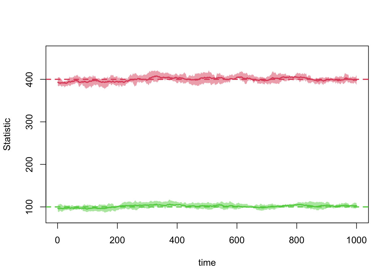

Code

plot(netdx_m1_d250_approx, mean.smooth = FALSE, qnts.smooth = FALSE)

Code

netdx_m1_d250_approx

EpiModel Network Diagnostics
=======================
Diagnostic Method: Dynamic
Simulations: 10
Time Steps per Sim: 1000

Formation Diagnostics
----------------------- 
           Target Sim Mean Pct Diff Sim SE Z Score SD(Sim Means) SD(Statistic)
edges         400  399.764   -0.059  1.971  -0.120         9.323        15.608
concurrent    100  101.459    1.459  1.348   1.082         6.059         9.968

Duration Diagnostics
----------------------- 
      Target Sim Mean Pct Diff Sim SE Z Score SD(Sim Means) SD(Statistic)
edges    250  249.839   -0.064  1.822  -0.088         7.598        12.021

Dissolution Diagnostics
----------------------- 
      Target Sim Mean Pct Diff Sim SE Z Score SD(Sim Means) SD(Statistic)
edges  0.004    0.004    0.574      0    0.73             0         0.003

The plots suggest that our statistics are hitting their targets nicely, a fact also confirmed by the Z scores in the printed netdx object.

Normally we might not bother to check the static diagnostics after seeing that the dynamic ones are good. We do so here for completeness and comparison to later examples:

Code

netdx_stat_m1_d250_approx <- netdx(est_m1_d250_approx, dynamic = FALSE, nsims = 1e3)


Network Diagnostics
-----------------------
- Simulating 1000 networks
- Calculating formation statistics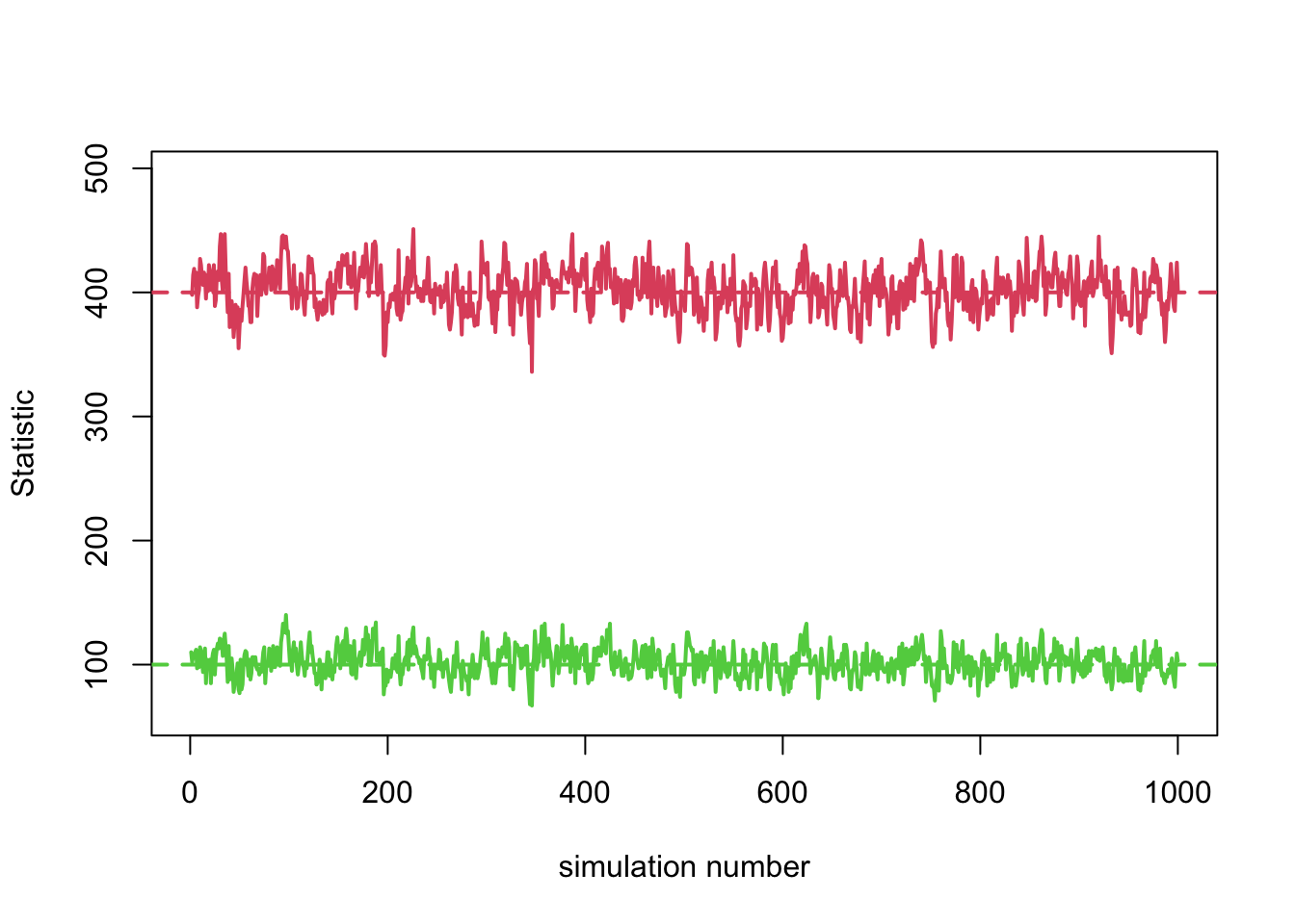

Code

plot(netdx_stat_m1_d250_approx, mean.smooth = FALSE)

Not surprisingly, these also look good.

54.3.2 Adding model complexity

We now try a model that starts to get a bit closer to the level one might see in some research-level projects. We will fully specify the momentary degree distribution, with a maximum degree constraint, and also add in selective mixing based on age. For the degree distribution, we include model terms for degrees 2 and 3, and specify a maximum degree of 3. We do not include terms for degrees 0 and 1, because with just the two already in there the model is fully specified, given additional features (total number of nodes, total number of edges). Age comes in many integer values here rather than a small number of categories, making absdiff a logical choice. Just remember that, given its definition, absdiff works differently than other categorical mixing terms, here a preference for similarity ends up leading to a negative coefficient, as the age difference within relationships will be less than expected by chance.

Our resulting model form and target statistics are:

Code

formation_m2 <- ~edges + degree(2) + degree(3) + absdiff("age")
target_stats_m2 <- c(400, 90, 10, 2000)

The expected number of edges is 400, and the total of the age differences within relationships is 2000; thus, on average a relationship will involve an age difference of 5 years. Considering that the population is spread out evenly over a 48-year age range (18 to 65), this is obviously quite a bit smaller than one would expect by chance. (Bonus question: what would you expect by chance? Hint: it’s not 48/2 = 24).

We mentioned a maximum degree constraint of 3, so you may have expected to see it here, as the model term degrange(from=4) with corresponding target statistic 0. That is one method for specifying degree constraints, and the one we emphasize in our introductory teaching materials. We do so because it means one less thing to learn about early on, and it works perfectly fine for simpler models that fit easily, and even for most larger and more complex models. However, as we dive into more advanced modeling it is worth learning an alternative approach: using the constraints argument during the call to netest. This method is more direct, as it formally sets the constraint a priori rather than having the algorithm detect the boundary condition and then set the coefficient to -Inf. This constrains the space that the MCMC can explore, adding a small boost of efficiency.

The syntax for a maximum degree constraint of X is bd(maxout=X), with the “out” simply a holdover from directed networks. Formal constraints use R formula notation since one can combine multiple constraints arbitrarily. For more information on constraints, see ?ergmConstraint.

This yields:

Code

set.seed(1)
system.time(
  est_m2_d250_approx <- netest(nw, formation = formation_m2,
                               target.stats = target_stats_m2, 
                               coef.diss = coef_diss_d250,
                               constraints = ~bd(maxout = 3)
                              )
            )

   user  system elapsed 
  0.883   0.017   0.900

Code

summary(est_m2_d250_approx)

Call:
ergm(formula = formation, constraints = constraints, offset.coef = coef.form, 
    target.stats = target.stats, eval.loglik = FALSE, control = set.control.ergm, 
    verbose = verbose, basis = nw)

Monte Carlo Maximum Likelihood Results:

             Estimate Std. Error MCMC % z value Pr(>|z|)    
edges       -3.831367   0.140217      0  -27.32   <1e-04 ***
degree2     -1.844489   0.143764      0  -12.83   <1e-04 ***
degree3     -3.619295   0.350036      0  -10.34   <1e-04 ***
absdiff.age -0.170519   0.009917      0  -17.19   <1e-04 ***
---
Signif. codes:  0 '***' 0.001 '**' 0.01 '*' 0.05 '.' 0.1 ' ' 1


Dissolution Coefficients
=======================
Dissolution Model: ~offset(edges)
Target Statistics: 250
Crude Coefficient: 5.517453
Mortality/Exit Rate: 0
Adjusted Coefficient: 5.517453

Code

netdx_m2_d250_approx <- netdx(est_m2_d250_approx, nsims = 10, nsteps = 1000, 
                              nwstats.formula = ~ edges + degree(0:5) + absdiff("age")
                              )

Code

netdx_m2_d250_approx

EpiModel Network Diagnostics
=======================
Diagnostic Method: Dynamic
Simulations: 10
Time Steps per Sim: 1000

Formation Diagnostics
----------------------- 
            Target Sim Mean Pct Diff Sim SE Z Score SD(Sim Means) SD(Statistic)
edges          400  398.801   -0.300  1.301  -0.921         3.070        11.524
degree0         NA  312.730       NA  1.838      NA         4.250        17.129
degree1         NA  586.901       NA  1.782      NA         5.317        17.216
degree2         90   90.407    0.452  1.178   0.346         3.305         9.944
degree3         10    9.963   -0.373  0.250  -0.149         1.133         2.733
degree4         NA    0.000       NA    NaN      NA         0.000         0.000
degree5         NA    0.000       NA    NaN      NA         0.000         0.000
absdiff.age   2000 2011.002    0.550 14.754   0.746        67.278       112.745

Duration Diagnostics
----------------------- 
      Target Sim Mean Pct Diff Sim SE Z Score SD(Sim Means) SD(Statistic)
edges    250  249.911   -0.036  1.674  -0.053         5.025        11.265

Dissolution Diagnostics
----------------------- 
      Target Sim Mean Pct Diff Sim SE Z Score SD(Sim Means) SD(Statistic)
edges  0.004    0.004    1.607      0   1.947             0         0.003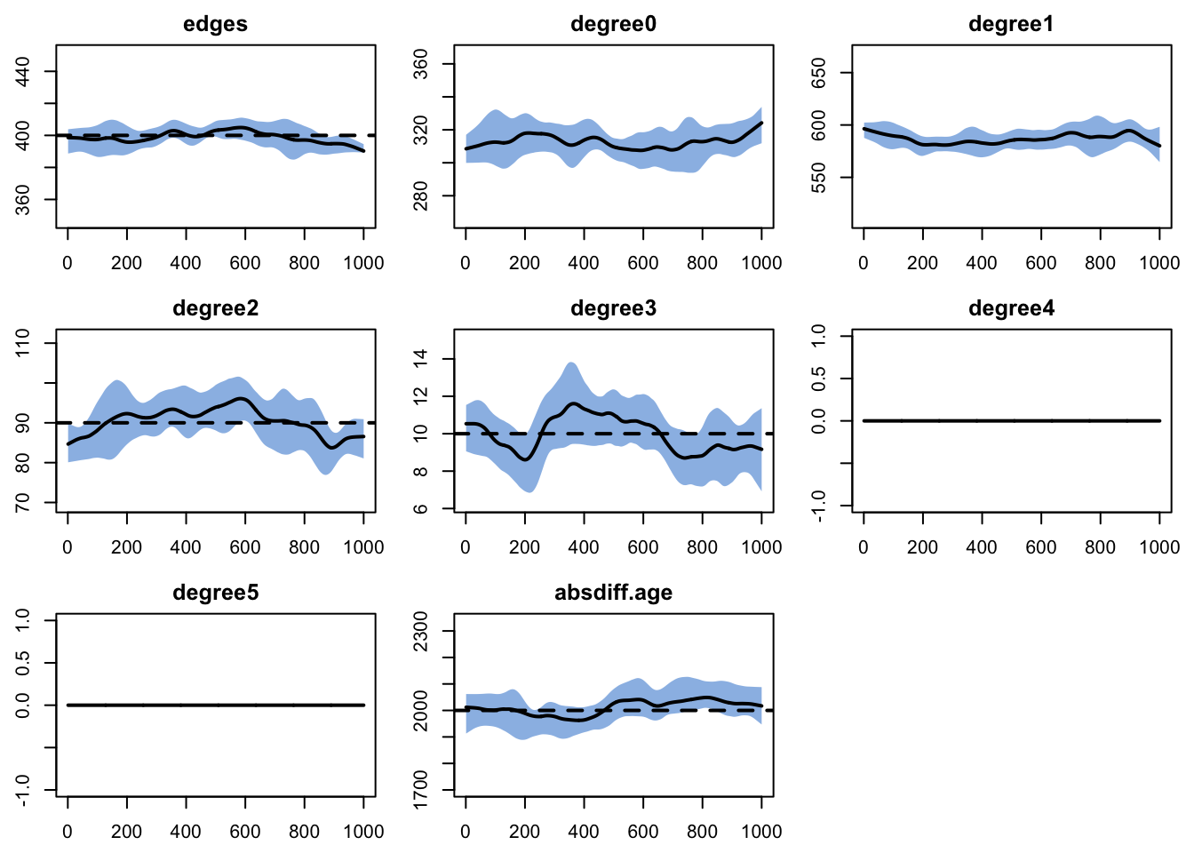

Code

plot(netdx_m2_d250_approx)

This model also fits well; diagnostics are generally as expected.

A key principle that these examples help illustrate is that the edges dissolution approximation method tends to work best for models with long mean relational durations. A general rule of thumb is that for a mean relationship duration above roughly 75-100, the approximation method is often all that one needs. This doesn’t hold true across all models and network sizes, and one should always check the diagnostics on one’s specific model to be sure. But it is a helpful guide to keep in mind.

Also remember that the time unit in models is arbitrary. This suggests an option if one is ever having trouble making a particularly complicated model with short relational durations fit. One can always re-define the time unit to a smaller measure, thus increasing the mean relational duration in time steps. Of course, one needs to remember to then change every time-based parameter throughout the epidemic model appropriately as well. One also needs to be prepared for longer simulation times. But the option is always there if needed.

Before going down that road, of course, one will generally want to try a full TERGM estimation, with its set of tune-able fitting parameters. We explore those next.

54.4 Conducting a full TERGM estimation

54.4.1 TERGM estimation with default parameters

We return to Model 1, our simple model with just edges and concurrent terms, but we try estimating it with a mean relational duration of 25 instead. Let’s see what happens if we use the approximation here:

Code

set.seed(1)
coef_diss_d25 <- dissolution_coefs(~offset(edges), 25, 0)

est_m1_d25_approx <- netest(nw, formation = formation_m1, 
                            target.stats = target_stats_m1, 
                            coef.diss = coef_diss_d25,
                            verbose = FALSE)
netdx_m1_d25_approx <- netdx(est_m1_d25_approx, nsims = 10, nsteps = 1000)


Network Diagnostics
-----------------------
- Simulating 10 networks
 |**********|
- Calculating formation statistics

Code

netdx_m1_d25_approx

EpiModel Network Diagnostics
=======================
Diagnostic Method: Dynamic
Simulations: 10
Time Steps per Sim: 1000

Formation Diagnostics
----------------------- 
           Target Sim Mean Pct Diff Sim SE Z Score SD(Sim Means) SD(Statistic)
edges         400  394.099   -1.475  1.045  -5.645         4.722        17.385
concurrent    100  100.670    0.670  0.775   0.865         3.249        11.418

Duration Diagnostics
----------------------- 
      Target Sim Mean Pct Diff Sim SE Z Score SD(Sim Means) SD(Statistic)
edges     25   24.936   -0.258  0.079  -0.811         0.225           1.2

Dissolution Diagnostics
----------------------- 
      Target Sim Mean Pct Diff Sim SE Z Score SD(Sim Means) SD(Statistic)
edges   0.04     0.04    0.358      0   1.481             0          0.01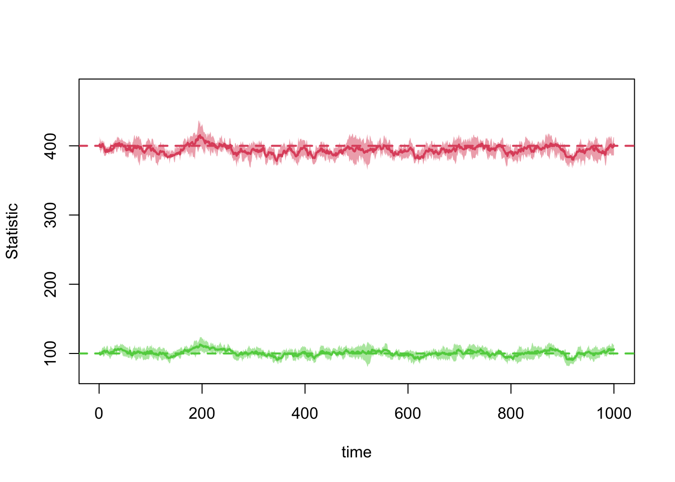

Code

plot(netdx_m1_d25_approx, mean.smooth = FALSE, qnts.smooth = FALSE)

We definitely see some small but consistent bias here. The number of edges in the diagnostic simulation now averages about 394.1, which is 1.5% too low. The plot makes it clear that this is reasonably consistent over time, and is not the result of some transitory stochastic bump. Interestingly the concurrent term seems to be much closer to its target, relatively.

Depending on their purposes, a modeler might decide that being off consistently by this small amount is acceptable. But let’s assume that they wish to try to improve the fit. In this case, the best thing to do next is to check the static diagnostics:

Code

netdx_stat_m1_d25_approx <- netdx(est_m1_d25_approx, dynamic = FALSE, nsims = 1e3)


Network Diagnostics
-----------------------
- Simulating 1000 networks
- Calculating formation statistics

Code

netdx_stat_m1_d25_approx

EpiModel Network Diagnostics
=======================
Diagnostic Method: Static
Simulations: 1000

Formation Diagnostics
----------------------- 
           Target Sim Mean Pct Diff Sim SE Z Score SD(Sim Means) SD(Statistic)
edges         400  399.804   -0.049  1.058  -0.185            NA        16.805
concurrent    100  100.780    0.780  0.721   1.082            NA        11.107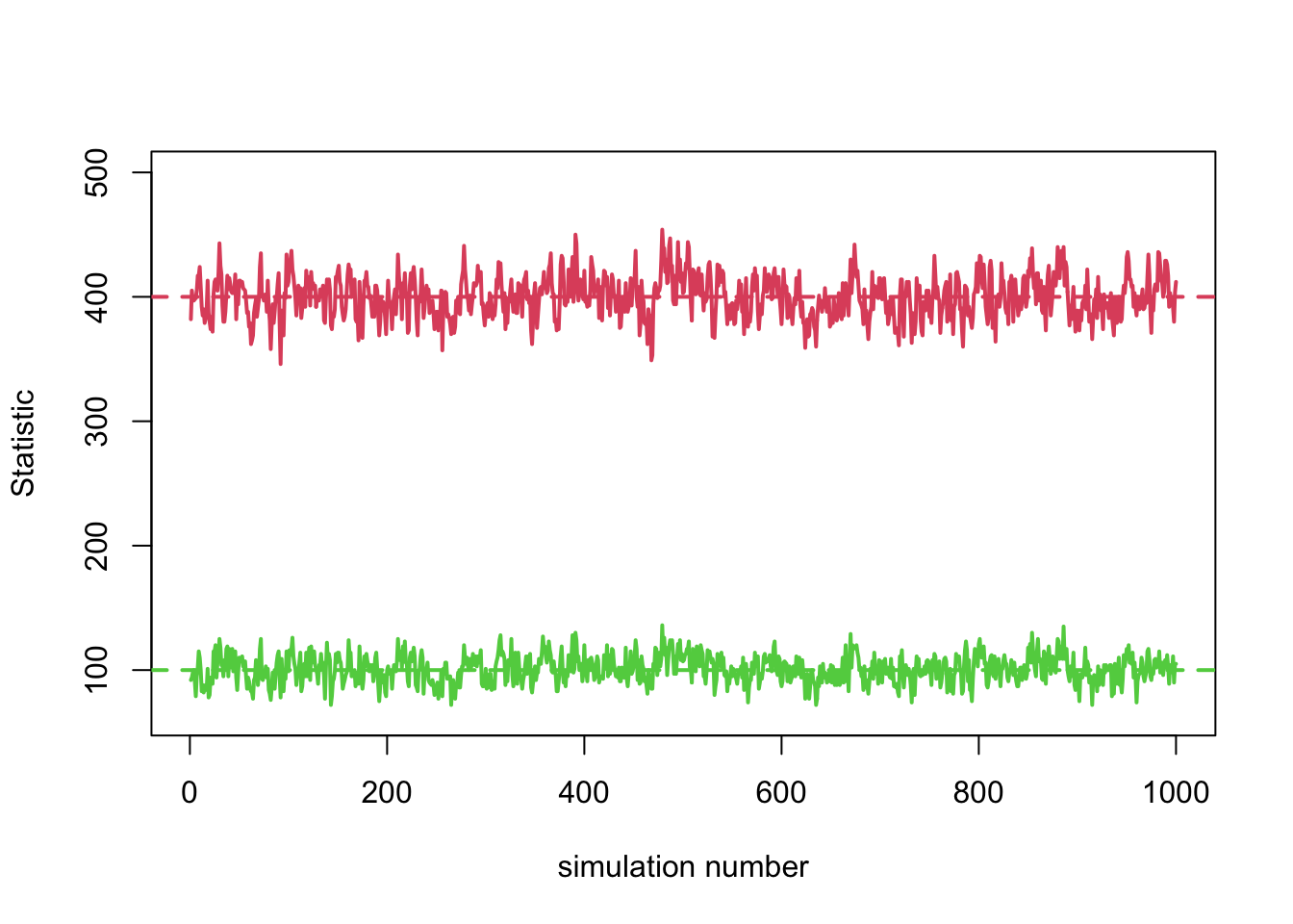

Code

plot(netdx_stat_m1_d25_approx, mean.smooth = FALSE)

These look very good, both in the table and the plot.

Poor dynamic diagnostics and good static diagnostics suggest that the use of edapprox is the most likely culprit. Our next step is clear: to re-run the model estimation with the approximation turned off and using full TERGM estimation instead (edapprox = FALSE). For now, we use all of the default fitting parameters for that process.

We are going to track how long it takes R to run this code, for comparison to later fits. If you are not familiar with this syntax, the command beginning with est_m1_d25_tergm will run normally, while the amount of time in seconds that it takes to run will be stored in the object est_m1_d25_tergm_time.

Code

set.seed(1)
est_m1_d25_tergm_time <- system.time(
  est_m1_d25_tergm <- netest(nw, formation = formation_m1, target.stats = target_stats_m1, 
                 coef.diss = coef_diss_d25, edapprox = FALSE
                   )
)

est_m1_d25_tergm_time

   user  system elapsed 
 97.096   0.182  97.362

Code

netdx_m1_d25_tergm <- netdx(est_m1_d25_tergm, nsims = 10, nsteps = 1000)


Network Diagnostics
-----------------------
- Simulating 10 networks
 |**********|
- Calculating formation statistics

Code

netdx_m1_d25_tergm

EpiModel Network Diagnostics
=======================
Diagnostic Method: Dynamic
Simulations: 10
Time Steps per Sim: 1000

Formation Diagnostics
----------------------- 
           Target Sim Mean Pct Diff Sim SE Z Score SD(Sim Means) SD(Statistic)
edges         400  401.354    0.339  1.075   1.259         3.969        17.577
concurrent    100  100.671    0.671  0.833   0.806         2.439        11.668

Duration Diagnostics
----------------------- 
      Target Sim Mean Pct Diff Sim SE Z Score SD(Sim Means) SD(Statistic)
edges     25   24.999   -0.005  0.085  -0.015         0.312         1.238

Dissolution Diagnostics
----------------------- 
      Target Sim Mean Pct Diff Sim SE Z Score SD(Sim Means) SD(Statistic)
edges   0.04     0.04   -0.166      0  -0.679             0          0.01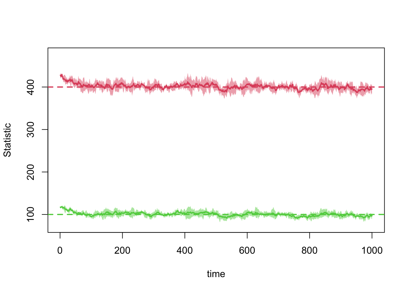

Code

plot(netdx_m1_d25_tergm, mean.smooth = FALSE, qnts.smooth = FALSE)

The summary table indicates that we are much closer now, and well within the normal margin of error, given the low Z scores. And to get there, the algorithm took 97.4 seconds, or roughly 1.6 minutes. The plot largely tells the same story, with one interesting new detail: the simulation seems to begin a little bit away from the target, but then move quickly towards it. Why do you think that might that be?

To understand the answer, it helps to dive into one specific element that you learned about earlier: that before starting the MCMC, one must “set a starting value for your vector of coefficients, $\theta$.” This actually involves two parts:

Generating a network that is reasonably close to the target statistics.
Using some tractable means to get an approximate value for $\theta$.

The first step is needed because we never directly created a network that had the observed target statistics; we just passed an empty network and told the algorithm what those targets were.

Neither of those steps needs to be perfect; they just need to be good enough to get one going, with the MCMC then refining the estimate repeatedly. That said, the closer one can get to the true MLE with this initial approximation, the easier a time the algorithm should have, and the quicker it should take.

By default, the network generation step uses a method called “simulated annealing”, or SAN. Remember, the algorithm doesn’t yet have access to the set of coefficients that would allow it to simulate networks from our model perfectly; those are precisely the coefficients we are working to estimate! So SAN is a bit more of a brute force algorithm, not guaranteed to get the exact network, but typically “good enough.” (And indeed, if your target statistics contain values that are possible as expected values but not possible for a single network (e.g., 34.6 edges), then it certainly cannot hit the target exactly). Estimation of starting values for $\theta$ that are “good enough” is then by default conducted using “maximum pseudolikelihood estimation”, or MPLE, via logistic regression.

The simulation you are seeing in the netdx_m1_d25_tergm plot, and all netdx plots, begins with that SAN-derived network. It can thus be off by a bit; and the more complex the model, the more likely it is to be off by a noticeable amount.

This is why it can be especially helpful to check not just the diagnostics table but also the plot; if this initial “slide” is big enough, it could generate Z-scores that suggest a problem, when the visual makes clear that the model is actually hitting its targets well.

Note that the same “slide” will be present in the epidemic simulation; if it is large enough that the user wishes to avoid it, then they will need to run a short burn-in first.

What happens if one tries to fit static diagnostics for this model?

Code

netdx_stat_m1_d25_tergm <- netdx(est_m1_d25_tergm, dynamic = FALSE, nsims = 1e3)

Error in netdx(est_m1_d25_tergm, dynamic = FALSE, nsims = 1000) : cannot perform static simulation without edapprox

One is reminded that static diagnostics are only a feature of a model fit with the edges dissolution approximation (edapprox = TRUE). Their main function is to confirm whether or not that approximation is the source of any observed issues; once the approximation is not being used, they are no longer defined.

Here are two additional scenarios that you can run to confirm that each also fits poorly with the approximation but well with TERGM estimation with default parameters:

A. Model 2 (full degree dist, age mixing), with mean relational duration of 25
B. Model 1 (edges + concurrent), with mean relational duration of 10

Together these suggest that, on the whole, TERGM estimation with its defaults can handle models with a good number of terms and/or mean relational durations that are quite short in terms of number of time steps, at least for networks of the size that we’ve considered here. Now we consider options when things don’t go quite so smoothly.

54.4.2 Refining TERGM estimation: MCMC burnin length

We consider a case where TERGM estimation fails with the default settings: model 2 with the relational duration of 10. Because of this we have the code commented out here:

Code

#set.seed(1)
#coef_diss_d10 <- dissolution_coefs(~offset(edges), 10, 0)
#est_m2_d10_tergm_time <- system.time(
#  est_m2_d10_tergm <- netest(nw, formation = formation_m2, target.stats = target_stats_m2, 
#                 coef.diss = coef_diss_d10, edapprox = FALSE
#                   )
#)

Un-commenting the above code and running it with the set-up we have on our machine eventually yields the error:

Error in solve.default(t(G) %*% w %*% G) : system is computationally singular

However, with other seeds the algorithm is sometimes able to succeed, but not consistently.

In our experience, the best place for users to start refining tergm estimation is with a pair of parameters called EGMME.MCMC.burnin.min and EGMME.MCMC.burnin.max. Earlier we mentioned that the core of the ERGM MCMC estimation algorithm needs to be repeated multiple times per time step within TERGM estimation. These two parameters govern what “multiple times” means in this case. By default, the algorithm aims to use information gathered during the process to adapt some elements of the algorithm as it goes, including this one. But sometimes the user is actually better able to use intuition and basic logic to fix that number. When one sets the min and max parameters to the same value, then the algorithm will use that exact value instead of trying to adapt. This can allow for increased algorithmic stability when it is most needed.

We find that a value of 1e4 (i.e. 1x10^4, i.e. 10k) works well on small networks like this one; for larger networks, it can be good to set it to something either on the same order of magnitude as the network size, or one larger. (Our network here has 1e3 nodes, so starting with 1e4 fits this rule of thumb, but one generally shouldn’t go much lower than 1e4 even if the network is much smaller).

The syntax for setting these parameters involves a function called control.tergm, which generates an object that then gets passed into netest with the argument set.control.tergm:

Code

control_tergm_b1e4 <- control.tergm(EGMME.MCMC.burnin.min = 1e4, 
                                    EGMME.MCMC.burnin.max = 1e4)
 
set.seed(1)
coef_diss_d10 <- dissolution_coefs(~offset(edges), 10, 0)
est_m2_s10_tergm_b1e4_time <- system.time(
    est_m2_s10_tergm_b1e4 <- netest(nw, formation = formation_m2, 
                                     target.stats = target_stats_m2, 
                                     coef.diss = coef_diss_d10, 
                                     edapprox = FALSE,
                                     set.control.tergm = control_tergm_b1e4
                                     )
    )

est_m2_s10_tergm_b1e4_time

Our estimation process ran fully with no error this time, taking about 13.6 minutes.

Crucially, setting the burn-in length during estimation means that one should also set it during simulation, both for diagnostics and full epidemic simulation. This is done by a call to the function control.simulate.formula.tergm (notice the added “simulate.formula” in the name), similarly passed in to set.control.tergm. There is one wrinkle here, though. By default, netdx sets one control parameter using this method: MCMC.maxchanges, which it sets to the largest integer the computer can handle using an internal R function. (One can see this at ?netdx). Users must re-iterate this entry if they are calling the function to set anything else; otherwise, it is lost:

Code

control_tergm_b1e4_sim <- control.simulate.formula.tergm(MCMC.burnin.min = 1e4,
                               MCMC.burnin.max = 1e4,
                               MCMC.maxchanges = .Machine$integer.max
                               )

netdx_m2_s10_tergm_b1e4 <- netdx(est_m2_s10_tergm_b1e4, 
                                    nsims = 10, nsteps = 1000,
                                    set.control.tergm = control_tergm_b1e4_sim
)


Network Diagnostics
-----------------------
- Simulating 10 networks
 |**********|
- Calculating formation statistics

Code

netdx_m2_s10_tergm_b1e4

EpiModel Network Diagnostics
=======================
Diagnostic Method: Dynamic
Simulations: 10
Time Steps per Sim: 1000

Formation Diagnostics
----------------------- 
            Target Sim Mean Pct Diff Sim SE Z Score SD(Sim Means) SD(Statistic)
edges          400  403.426    0.857  1.279   2.678         6.052        22.928
degree2         90   90.258    0.287  0.293   0.880         1.440        10.066
degree3         10   10.360    3.601  0.133   2.716         0.584         3.545
absdiff.age   2000 2027.051    1.353  9.735   2.779        39.345       169.668

Duration Diagnostics
----------------------- 
      Target Sim Mean Pct Diff Sim SE Z Score SD(Sim Means) SD(Statistic)
edges     10   10.005    0.054  0.019   0.288         0.043         0.464

Dissolution Diagnostics
----------------------- 
      Target Sim Mean Pct Diff Sim SE Z Score SD(Sim Means) SD(Statistic)
edges    0.1      0.1   -0.044      0    -0.3             0         0.015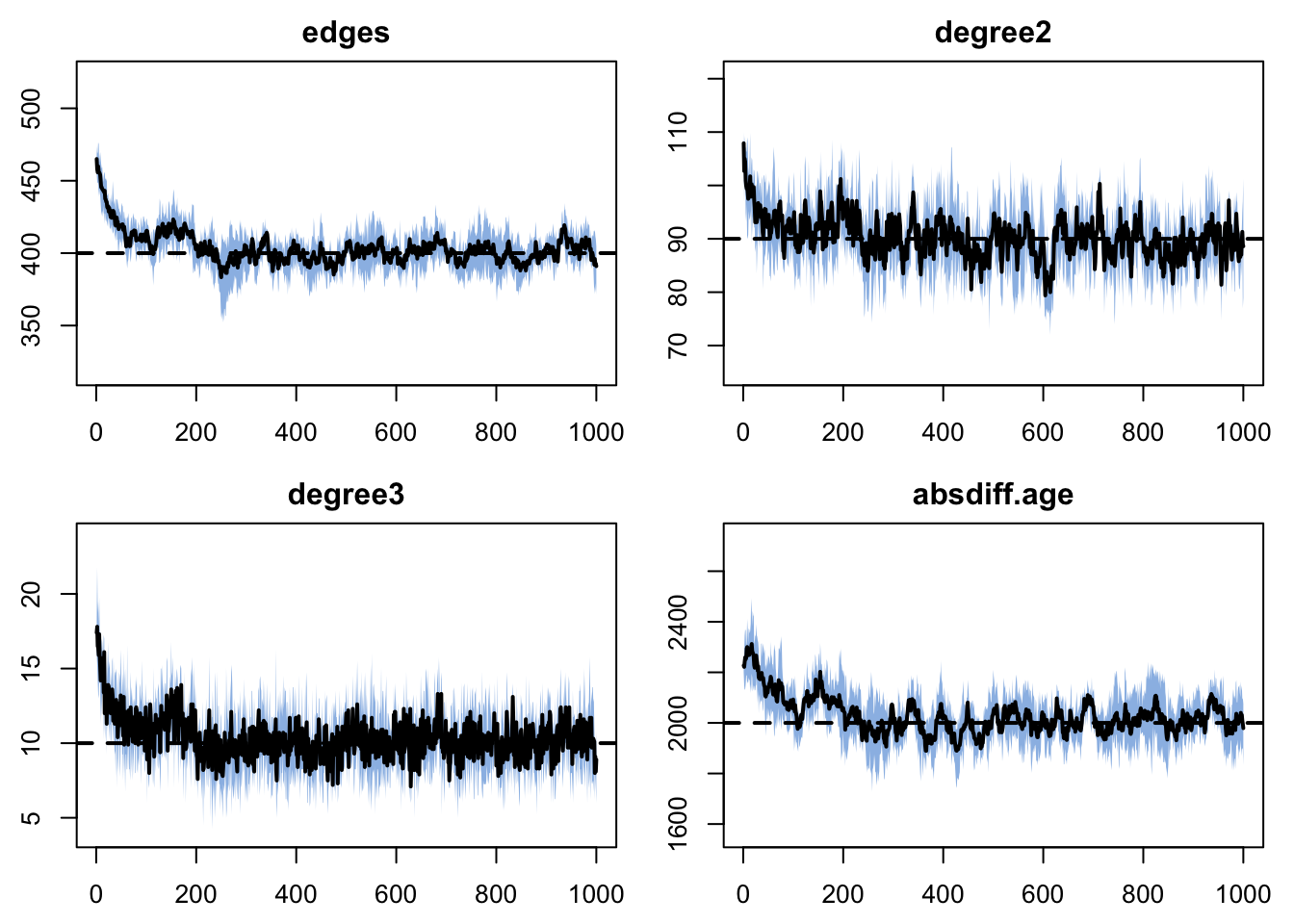

Code

plot(netdx_m2_s10_tergm_b1e4, mean.smooth = FALSE, qnts.smooth = FALSE)

So the model fits well, albeit again with the “SAN slide” at the beginning.

Try running these diagnostics without setting the MCMC.burnin length and just letting the algorithm use the default. You should see the simulation yield networks that have too few edges, as the algorithm does not have sufficient steps to get up from an empty network to the correct density.

54.4.3 Table of commonly used TERGM fitting parameters

TERGM has a great many fitting parameters, viewable at tergm::control.tergm. However, in our experience, a few turn out to be the most important in practice for these types of models. These are:

Parameter	Notes
`EGMME.MCMC.burnin.min`, `EGMME.MCMC.burnin.max`	Sets the length of the MCMC burn-in. The default algorithm attempts to set this length dynamically but can face challenges. Setting these two parameters to the same value forces a specific burn-in length. Useful values to start with are `1e4` or the number of nodes in the network, whichever is larger.
`SAN.maxit`	Sets the maximum number of iterations during simulated annealing. Larger values can help get a network closer to the target statistics. Default is 4; one commonly used value is 20.
`MCMC.prop = ~sparse`	A “hint” that tells the algorithm the network is sparse, and to use a sampling regime optimized for that condition. See `?ergmHint`. Note this one is in effect by default. Hints use formula notation and can be combined; if you add other hints, include this one explicitly as well to ensure it does not get dropped. Requires no value, just the hint name `sparse`.
`MCMC.prop = ~discord`	A “hint” that it would be useful to over-sample from dyads already toggled during the current MCMC chain, raising their sampling proportion to around 50%. Requires no value, just the hint name `discord`.
`MCMC.prop.args = list(discordance_fraction)`	An alternative way to set directly the proportion of times a previously toggled dyad is selected. Can be set to any value between 0 and 1. In practice 0.5 is the benchmarked default and we rarely move it; the simulation-stage table below treats discordance proposals more fully.
`MCMC.prop = ~strat(attr, empirical = TRUE)`	A “hint” telling the algorithm how often to select different sets of dyads for possible toggling. Very useful where large proportions of dyads are impossible or very unlikely. For example, a population in which most ties are between nodes sharing an `age.group` value can be made much more efficient with `MCMC.prop = ~strat(attr = "age.group", empirical = TRUE)`.
SAN proposals, via the `SAN` sub-control	SAN inherits its proposal from `MCMC.prop` automatically, so there is no top-level `SAN.prop` argument; passing one is an error. To give SAN a different proposal, pass a whole sub-control object: `control.tergm(SAN = control.san(SAN.prop = ~strat(attr = ~race, pmat = Y)))`.

Note: it is possible to use more than one MCMC.prop hint; simply combine them with R’s formula notation, e.g., MCMC.prop = ~sparse + discord + strat(attr = "race", empirical = TRUE)

54.5 Fine-tuning ERGM estimation

As we saw earlier, there are many cases (especially with long relationship durations) where EpiModel users can rely on the edge duration approximation for final model coefficients. This requires performing ERGM estimation only, which is generally much easier and faster than TERGM estimation. This is not to say that ERGM estimation is always easy and fast, however. Learning how to fine-tune ERGM estimation with fitting parameters is just as important as for TERGM. Indeed, for larger and larger networks, fitting a TERGM becomes increasingly difficult, and in our experience most users end up relying on the approximation at this scale most of the time. This may include re-defining the time step in the model to a shorter unit as part of the process.

The set of fitting parameters available for ERGMs can be seen at ergm::control.ergm. Parallel to TERGMs, these are passed as arguments in a call to control.ergm, which creates an object that is then passed into EpiModel’s netest with the argument set.control.ergm.

The subset commonly modified during epidemic modeling is reasonably small, and the table below is the merged shortlist: the parameters we vary out of the box, plus the ones we reach for when a fit misbehaves. In our own applied models (some of which are very large and very complex) these cover roughly 95% of our use cases.

Parameter	What it does	When to reach for it
`main.method`	Selects the estimation method used to find the MLE: `"MCMLE"` (the default, robust, what we use on HPC) or `"Stochastic-Approximation"` (fast, good for small or dyad-independent models fit locally).	Flip to Stochastic-Approximation for quick local fits; keep MCMLE for the production fit. SA can over- or under-recover on large networks, so verify with `netdx`.
`MCMLE.maxit`	Maximum number of times the MCMC parameter is updated by maximizing the MCMC likelihood. Default is 60.	Raise for a slow, hard fit; the model may need many iterations to settle. 200 to 500 is the useful range, and we commonly use 500.
`MCMC.samplesize`	Number of network statistics recorded during each MCMC iteration. Default is determined adaptively.	The single biggest cost lever. A smaller sample (for example `1e4` rather than `5e4`) makes every iteration cheap, which can turn a fit that pegs the cores for a day into one that finishes in minutes. To stop ergm adapting the sample size out from under you, set `MCMLE.effectiveSize = NULL` (its default is 64); `MCMC.effectiveSize` is already `NULL` by default, so setting it changes nothing.
`MCMC.interval`	Number of MCMC proposal steps between networks whose statistics are recorded in the sample (thinning). Default is determined adaptively.	Raise to reduce autocorrelation between draws on a slow-mixing chain; lower to sample more densely. A common starting value is `5e3`.
`MCMC.burnin`	Burn-in steps before the first retained draw each iteration.	Raise for large or slow-mixing networks. A rule of thumb from practice: at least the same order of magnitude as the network size.
`MCMC.maxedges`	Hard ceiling on the number of edges in an MCMC draw. Defaults to `Inf`, so by default there is no ceiling at all.	Set a tight finite value so a degenerate, runaway draw fails fast with a status error instead of mixing slowly for hours. The only default backstop is `MCMLE.density.guard` (`exp(3)`, about 20 times the observed edge count), and it engages only once a draw exceeds `MCMLE.density.guard.min` of 10,000 edges, so on a dense fit there is effectively nothing catching you. One of the highest-value and least-obvious controls.
`MCMLE.steplength` + `MCMLE.steplength.margin`	The optimization step length, and whether it is a pinned value or a ceiling.	To keep iteration 1 from lunging into a bad region, pin the step: set `MCMLE.steplength = 0.5` and `MCMLE.steplength.margin = NULL`. The `margin = NULL` is load-bearing and non-obvious: with the default margin, `steplength` is only the maximum and ergm’s Hummel search raises the actual step toward it, so setting `steplength` alone does not pin anything.
`MCMLE.termination`	The rule for stopping between iterations: `"confidence"` (the default) or `"Hummel"`.	Use `"Hummel"` to avoid the between-iteration sample-size blow-up that `"confidence"` triggers on a hard fit. Note it requires `steplength = 1` with a non-null margin, so it cannot be combined with a pinned step; pick one strategy or the other.
`SAN.maxit`	How many annealing iterations the fixed SAN budget is split across. It does not change total SAN effort. Default is 4.	Raise (12 to 20) for a finer-grained anneal toward the targets, but pair it with a raised `SAN.nsteps.times`, or each iteration simply gets a smaller share.
`SAN.nsteps.times`	The total SAN budget, as a multiplier on `MCMC.burnin` (`SAN.nsteps = SAN.nsteps.times * MCMC.burnin`). The `ergm` documentation calls this arguably the most important of the SAN parameters. Default is 8.	Start at the default and ramp up, to 16 or beyond, when SAN is failing to reach the targets. Watch the multiplier: `MCMC.burnin` is itself derived from `MCMC.interval`, so changing that silently rescales SAN too.
`init.MPLE.samplesize`	Sample size for the MPLE that seeds MCMLE.	Raise for a better starting point on a large or complex model.
`MCMC.prop`	The MCMC proposal distribution. The ergm default is `~sparse + .triadic`; tergm’s is `~discord + sparse`. Hints combine with formula notation, and listing any hint replaces the default, so re-list the ones you still want.	Use `~strat(...) + sparse` when the sampler is starving rare or empty regions of the mixing matrix (few contacts among some age or race cells): it passes a matrix of sampling weights so the chain stops repeatedly proposing in near-empty cells. Often the fastest fix on a dense, structured network. SAN inherits this proposal automatically.
`parallel`	Number of parallel MCMC chains and cores. The MCMC sample is divided across cores.	Raise on an HPC node. Depends on available hardware; `parallel::detectCores()` reports what you have.

These two deserve a note together, because the relationship is not the obvious one. SAN.nsteps.times is the only lever on total SAN effort: it sets SAN.nsteps = SAN.nsteps.times * MCMC.burnin, which defaults to 8 * 16,384 = 131,072 steps. SAN.maxit does not add to that budget, it divides it: the total is allocated across that many annealing iterations under a decreasing schedule. Raising SAN.maxit alone therefore gives you more, shorter anneals rather than more work. If SAN is failing to reach the targets, raise SAN.nsteps.times.

The values above are close to the recipe we actually run in our production HIV models, which is a useful reference point for a large network:

control.ergm(
  main.method      = "MCMLE",   # "Stochastic-Approximation" for faster local fits
  MCMLE.maxit      = 500,
  SAN.maxit        = 3,
  SAN.nsteps.times = 4,
  MCMC.samplesize  = 1e4,
  MCMC.interval    = 5e3,
  parallel         = est_cores)

The SAN numbers there look smaller than the defaults, and this is a good illustration of why that reasoning misleads. Because MCMC.interval = 5e3 raises MCMC.burnin to 80,000, that recipe’s SAN.nsteps is 80,000 * 4 = 320,000, roughly 2.4 times the default of 131,072. The SAN is more thorough than the default, not less, despite the smaller-looking multiplier. Always resolve the product rather than reading the multiplier alone, and start from the defaults on a new model.

A compact example combining several of these, in the style we use for a large, structured fit:

est <- netest(nw, formation, target.stats, coef.diss,
              constraints = ~bd(maxout = 2),
              set.control.ergm = control.ergm(
                main.method       = "MCMLE",
                MCMC.samplesize   = 1e4,
                MCMC.maxedges     = 5e6,
                MCMLE.effectiveSize = NULL,
                MCMLE.steplength  = 0.5,
                MCMLE.steplength.margin = NULL,
                SAN.maxit         = 12,
                SAN.nsteps.times  = 16,
                MCMC.prop         = ~strat(attr = ~age.grp) + sparse,
                parallel          = 4))

54.6 Fine-tuning simulation

Network simulation is part of both network diagnostics (netdx) and epidemic simulation (netsim), and needs to be accounted for similarly in both. The process of simulation is generally more straightforward than estimation, but it still can require some tweaking of parameters. This is especially true on larger networks, since the number of MCMC steps needed grows with the amount of change the model has to produce, both at the outset and again at each time step. Note that simulation always involves TERGM, regardless of whether estimation was conducted with ERGM or TERGM. All of the same fitting parameters and recommended values mentioned under TERGM estimation thus apply here, with some important additional details:

If a parameter relating to the length of the MCMC chain is set during estimation, it is generally recommended to set the analogous parameter to the same value during simulation. We already saw one example of this above, where a change to both EGMME.MCMC.burnin.max and .min during TERGM estimation had to be paired with a similar change to MCMC.burnin.max and .min during simulation.
The MCMC.interval parameter for ERGM estimation is analogous to MCMC.burnin.max and .min during simulation, even though that relationship is not obvious from the names alone.
Here the fitting parameters are first passed as arguments to the function control.simulate.formula.tergm, which creates an object that is then passed into netdx or netsim with set.control.tergm.

The controls below are the ones we actually change at this stage. They are a common source of a fit that “looks broken” but is not: the model is fine and the stepping is what needs adjusting.

Parameter	What it does	When to reach for it
`MCMC.burnin.min`, `MCMC.burnin.max`	The per-step burn-in used when the network is re-simulated each time step.	Pin both (for example to `1e4`) for short-duration models. At a mean duration of 10, a tenth of edges dissolve every step, and the default per-step burn-in cannot re-form them back to target before the step ends, so edges come back low (for example around 390 against a target of 400, with a large negative Z score). Pinning the burn-in recovers the target. tergm has no `MCMC.interval`; setting `MCMC.burnin.min = MCMC.burnin.max` is how you fix the proposals per step.
`MCMC.maxchanges`	Ceiling on the number of toggles per simulation. Default is `1e6`, though `netdx` already raises it to `.Machine$integer.max`.	Raise (up to `.Machine$integer.max`) when a diagnostic or run hits a maxchanges error, or when a large, dense network needs many toggles to reach equilibrium.
`MCMC.prop = ~discord`, `discordance_fraction`	Discordance-focused proposals: the dynamic analogue of TNT, focusing toggles on dyads that have changed since the start of the step (the “sparse” set in a dynamic network). `discordance_fraction` (default 0.5) tunes how often a discordant dyad is proposed.	Use to improve mixing when the per-step change set is what is hard to sample. `~discord` is essentially `discordance_fraction = 0.5`; set `discordance_fraction` explicitly to pick another value. In practice 0.5 is the benchmarked default and we rarely move it.

Set the same controls in netsim, not just netdx

If pinning the per-step burn-in fixes your netdx diagnostics, pass the same set.control.tergm to netsim(). The production run steps the network with the same kernel, so without it the epidemic runs on the same under-mixed network the diagnostics flagged. This is not cosmetic.

54.7 Two diagnosis traps

Both of these cost real time because the obvious reading is wrong.

Do not blame the structural-zero cells. When a mixing matrix has empty cells (no school contacts for people over 60, for example), ergm 4.x already detects them (“Observed statistic(s) are at their smallest attainable values; their coefficients will be fixed at -Inf”) and handles them. They are not the cause of a stalled fit; the slow mixing is among the remaining free parameters. Adding an explicit constraint for them does not help.
“Static recovery looks terrible” is usually a burn-in artifact, not a bad fit. If you sanity-check a fit by simulating a static network from empty (netdx(..., dynamic = FALSE)) and the edges come back far short of target, suspect the diagnostic burn-in before the fit. From an empty start the default burn-in is nowhere near equilibrium, and the gap widens with network size. It is a gradient, not a cliff: raising the simulation MCMC.burnin recovers the same coefficients (edges recovered climbing from about 0.13 at default, to about 0.79 at 1e6, to about 0.99 at 1e7 on one large layer).

54.8 A worked recipe: a fit that stalled for a day

A concrete case that exercises most of the estimation shortlist. Fitting a dense, dyad-independent contact-network layer (per-capita fractional targets, several structural-zero age-mixing cells) with a reasonable-looking control (MCMC.samplesize = 5e4, default step, no MCMC.maxedges) pegged 16 cores at 98% for 23 hours without clearing iteration 2, while the structurally simpler companion network converged in under three hours. The stall was slow mixing after iteration 1 overshot into a bad region, under a loose default density guard.

The fixes all attacked the same two things, bound the per-iteration cost and stop iteration 1 from overshooting:

MCMC.samplesize = 1e4 (down from 5e4) plus MCMC.maxedges = 5e6: a small fixed sample makes every iteration cheap, and a tight finite maxedges turns a degenerate dense draw into a fast error rather than a slow draw. The single biggest lever.
MCMLE.steplength = 0.5 with MCMLE.steplength.margin = NULL: pins the step so iteration 1 cannot lunge.
MCMLE.termination = "Hummel" (as an alternative to the pinned step): terminates without the confidence sample blow-up.
MCMC.prop = ~strat(attr = ~age.grp) + sparse: fastest on the dense layer, where the sampler was starving the rare elderly cells.
SAN.maxit = 12, SAN.nsteps.times = 16: strong enough SAN that the MPLE exists on the structural-zero cells.

The worst case went from 23 hours of non-convergence to about 2.4 minutes. The layer’s character decides the best proposal: the small-sample plus Hummel recipe is fastest on sparse layers, the stratified proposal on dense ones. The transferable content is which controls matter and why; the literal magnitudes are tuned to a particular set of networks.

54.9 Two practical shortcuts

Constraining maximum degree. Start with degrange(from = k) and a target statistic of 0. It keeps the cap in the formation formula alongside every other target, which is one less concept to carry and is formulaically elegant: every structural feature of the model is expressed the same way. It is not necessarily the most computationally or mathematically optimal choice, though, and it does not need to be while the model is fitting comfortably. If you get stuck and find yourself tuning controls, that is the moment to switch to the formal constraint, constraints = ~bd(maxout = k) with the term carried as an offset, which bounds the space the MCMC explores a priori rather than letting the algorithm discover the boundary and drive the coefficient to -Inf.

Transferring a dyad-independent fit across network sizes. When the formation model is dyad-independent and the targets are per-capita, you can skip a large-N fit entirely: fit the model at a small population fraction (fast and stable, often with Stochastic-Approximation), then move the coefficients to the full network unchanged except the edges term, which shifts by log(N_small) - log(N_big) to hold mean degree fixed. This is exactly the open-population edges adjustment from Module 7.

theta <- coef(fit_small$fit)
theta["edges"] <- theta["edges"] + log(N_small) - log(N_big)  # differential terms unchanged

Simulating the large network from these transferred coefficients (with an adequate burn-in, per the trap above) recovers the targets to about 0.99, and an independent full fit lands on the same edges coefficient. It rests on the sparse plogis to exp approximation, which is why the recovery is approximate rather than exact.

54.1 Introduction

54.2 Setup

54.3 Refresher on default model estimation in netest

54.3.1 Simple model, small network, long relational durations

54.3.2 Adding model complexity

54.4 Conducting a full TERGM estimation

54.4.1 TERGM estimation with default parameters

54.4.2 Refining TERGM estimation: MCMC burnin length

54.4.3 Table of commonly used TERGM fitting parameters

54.5 Fine-tuning ERGM estimation

54.6 Fine-tuning simulation

54.7 Two diagnosis traps

54.8 A worked recipe: a fit that stalled for a day

54.9 Two practical shortcuts

54.3 Refresher on default model estimation in `netest`