# Appendix: How Fast Is the Network?
::: {.callout-note}
This appendix is optional, and it works differently from the tutorials. Where they teach by watching movies, it develops a single idea through diagnostics and small tables, so it sits outside the main sequence, after the lab. Read it if you are curious how the module's pieces fit together; nothing later in the course depends on it.
:::
Every tutorial in this module changed one feature of the network, concurrency, duration, clustering, heterogeneity, and watched what it did to an epidemic. This appendix steps back to the question underneath all of them: **how fast does the network turn over, relative to how fast the epidemic moves?** That single ratio, the network's clock against the epidemic's clock, decides which of those features matters and which is a detail, and naming it turns a catalogue of terms into one idea.
::: {.callout-note}
Download the R script to follow along [here](mod5-Timescale.R).
:::
## Two Clocks
An epidemic has a clock: the generation interval, the pace at which infection moves from one contact to the next (in this SI process with no recovery, simply how fast it advances along the network). A network has a clock too: how quickly partnerships form and dissolve, which we have been setting all module with the `duration` argument. The relationship between network epidemiology's two great traditions, and most of what is confusing about when to use which, is the ratio of these two clocks.
- When the **network clock is slow** relative to the epidemic (partnerships outlast the outbreak), the contact network is effectively frozen while the epidemic runs. Structure is destiny: who is reachable is fixed before the first case. This is the world of **percolation and the epidemic threshold**, the results the field built first.
- When the **network clock is fast** relative to the epidemic (partnerships turn over many times during the outbreak), the network rebuilds itself under the epidemic. Timing is everything, and the momentary network is a poor guide to who gets infected. This is the world of **rapid mixing and concurrency**.
You have already built both extremes, in the [duration tutorial](mod5-Timing.html): the very-long-duration run (a frozen network) and the one-step run (rebuilt every step). There we read them as two modeling traditions. Here we read them as the two ends of one dial, the clock ratio, and build the tools to tell which end a given model sits at.
## Setup
The same packages as the other tutorials, plus `sna` and `tsna` from the `statnet` suite, which give us the static and temporal network measures below. We reuse the animation helper and the fixed poker-chip SI epidemic.
```{r setup, message = FALSE, warning=FALSE}
library("EpiModel")
library("ndtv")
library("sna")
library("tsna")
library("htmlwidgets")

slice.par  <- list(start = 1, end = 25, interval = 1, aggregate.dur = 1, rule = "any")
render.par <- list(tween.frames = 10, show.time = FALSE)
plot.par   <- list(mar = c(0, 0, 0, 0))

animate <- function(sim) {
  nw <- get_network(sim)
  nw <- color_tea(nw, verbose = FALSE)
  compute.animation(nw, slice.par = slice.par, verbose = FALSE)
  render.d3movie(
    nw, render.par = render.par, plot.par = plot.par,
    vertex.cex = 0.9, vertex.col = "ndtvcol",
    edge.col = "darkgrey", vertex.border = "lightgrey",
    displaylabels = FALSE, output.mode = "htmlWidget")
}

movie.param   <- param.net(inf.prob = 1)
movie.init    <- init.net(i.num = 10)
movie.control <- control.net(type = "SI", nsteps = 25, nsims = 1)
```
## A Diagnostic: Momentary vs Cumulative Degree
Here is a concrete decision the clock ratio settles. Suppose you can vaccinate the 15 best-connected people in a population of 100. "Best connected" by which count: the number of partners someone has **right now** (their momentary degree), or the number they accumulate **over the course of the epidemic** (their cumulative degree)? On a slow network these are the same list. On a fast one they are almost unrelated, and picking the wrong one wastes the doses.
We can measure both directly. `network.collapse()` flattens a dynamic network to a static one: at a single instant (`at =`) it returns the momentary network, and over a window (`onset`, `terminus`) it returns the cumulative network, in which an edge exists if the pair was tied at any point in that window. `degree()` then counts partners in each. The helper fits an edges-only network at a given duration and simulates its dynamics over a horizon. We drive that simulation with `netdx` (asking it to keep the full dynamic network via `keep.tnetwork`) rather than `netsim`, because here we want the contact network's own behavior over time, with no epidemic running on it.
```{r deg-profile, message=FALSE, warning=FALSE}
degree_profile <- function(duration, horizon = 50, seed = 1234) {
  set.seed(seed)
  nw  <- network_initialize(100)
  est <- netest(nw, ~edges, 50,
                dissolution_coefs(~offset(edges), duration = duration),
                verbose = FALSE)
  dx  <- netdx(est, nsims = 1, nsteps = horizon, dynamic = TRUE,
               keep.tnetwork = TRUE, verbose = FALSE)
  nwd <- get_network(dx, sim = 1)
  data.frame(
    momentary  = degree(network.collapse(nwd, at = horizon), gmode = "graph"),
    cumulative = degree(network.collapse(nwd, onset = 1, terminus = horizon + 1),
                        gmode = "graph"))
}
```
We run it at two durations, both fit to a target mean degree of 1 (50 edges) over the same 50-step horizon: a slow network (mean duration 200 steps, four times the horizon) and a fast one (mean duration 2 steps, turning over about 25 times during it).
```{r deg-run, message=FALSE, warning=FALSE, results="hide"}
slow <- degree_profile(duration = 200)
fast <- degree_profile(duration = 2)
```
```{r deg-compare}
compare <- function(d) {
  top <- function(x) order(x, decreasing = TRUE)[1:15]
  data.frame(
    mean_momentary  = round(mean(d$momentary), 2),
    mean_cumulative = round(mean(d$cumulative), 2),
    correlation     = round(cor(d$momentary, d$cumulative), 2),
    top15_overlap   = length(intersect(top(d$momentary), top(d$cumulative))))
}
rbind(slow = compare(slow), fast = compare(fast))
```
On the **slow** network, momentary and cumulative degree are nearly the same number (about 1.0 and 1.2) and, more to the point, nearly the same people: the two vaccination lists share 13 of 15. Edges barely change, so whom you are with now is whom you will be with. On the **fast** network, momentary degree still sits near one (the 0.72 in the table is a single instant of a fast-churning network reading a bit below its target mean degree of one), but each person accumulates roughly 22 distinct partners over the horizon, the two measures correlate near zero, and the vaccination lists share only 3 of 15. Ranking people by their current partners tells you almost nothing about whom they will contact over the epidemic.
::: {.callout-note .concept}
## Which degree matters is a question about the clock ratio, not the disease
When the network is slow relative to the epidemic, momentary and cumulative degree collapse into one number, exactly as they do on the frozen network from the [duration tutorial](mod5-Timing.html), where no edge ever ends. When the network is fast, they diverge, and the cumulative measure is the one that tracks transmission. This is not a special fact about vaccination; it is the same collapse the frozen-network callout described, now read from the intervention side. The clock ratio decides whether the distinction is worth measuring.
:::
This is a live concern in applied work, not a classroom curiosity. In dynamic network models of respiratory pathogens fit to empirical contact data, prioritizing vaccination by a momentary degree measure versus a cumulative one can make little difference to the outcome, precisely because a fast respiratory epidemic running on a contact network that shifts only slowly sits at the slow end of this ratio, where the two measures nearly coincide. The clock ratio, rather than the intuition that "degree-based targeting just needs the right degree," is what tells you when the two measures part company.
::: {.callout-note .concept}
## Optional deepening: network turnover is incidence, and momentary degree is a prevalence
This aside connects the diagnostic to core epidemiology; nothing later in the appendix depends on it, so skip it on a first pass if you like. The two degree measures are a familiar epidemiologic identity in disguise. Partnerships have a prevalence and an incidence, just as infections do, linked by the same relation: prevalence equals incidence times duration, $P = I \times D$. The **momentary mean degree is the prevalence of partnerships**, how many exist at an instant. The **duration** is $D$, the argument we have dialed all module. Their ratio, momentary degree over duration, is the partnership **incidence**: the rate at which new ties form, which is the network's turnover, the network clock itself. Cumulative degree is then what that incidence delivers over the epidemic's lifetime, on the order of the momentary degree times the number of turnovers (horizon over duration). On the slow network, duration dwarfs the horizon, turnover is near zero, and cumulative barely exceeds momentary ($1.0 \times (1 + 50/200) = 1.25$ predicted, 1.24 observed). On the fast network, the same momentary prevalence is churned over about 25 times, so cumulative runs many-fold higher. Hold prevalence fixed and shorten duration, and you have raised incidence without touching prevalence, which is exactly the move from the slow network to the fast one. Turnover, the diagnostic, and the duration dial are three views of one identity.
:::
## The Slow Limit: The Epidemic Threshold
When the network clock is much slower than the epidemic, the network is frozen and the reachable set is the connected component a seed lands in. This is where network epidemiology's most famous result lives: the **epidemic threshold**. Below a critical mean degree, a random graph is a scatter of small components and no epidemic can take off; above it, a **giant component** appears that spans a finite fraction of the population, and an outbreak seeded anywhere in it can reach that whole fraction.
We can watch the threshold form. We freeze the network (duration 100,000, as in the duration tutorial), sweep the mean degree, and for each value measure two things: the size of the largest connected component on the static graph (`sna::component.dist`), and the epidemic's mean final size from a single seed with certain transmission. To get static graphs to measure, we reach for the fitted cross-sectional model that `netest` stores as `est$fit`: simulating from it (`simulate(est$fit, output = "network")`) draws individual networks from the same ensemble the epidemic runs on, and we average the giant-component fraction over twenty such draws.
```{r threshold-sweep, message=FALSE, warning=FALSE, results="hide"}
threshold_row <- function(edges, n = 100, nsims = 100, nsteps = 80) {
  set.seed(1234)
  nw  <- network_initialize(n)
  est <- netest(nw, ~edges, edges,
                dissolution_coefs(~offset(edges), duration = 1e5), verbose = FALSE)
  giant <- mean(replicate(20,
    max(component.dist(simulate(est$fit, output = "network"),
                       connected = "weak")$csize) / n))
  sim <- netsim(est, param.net(inf.prob = 1), init.net(i.num = 1),
                control.net(type = "SI", nsteps = nsteps, nsims = nsims,
                            ncores = 5, verbose = FALSE))
  final <- as.data.frame(sim)$i.num[as.data.frame(sim)$time == nsteps]
  data.frame(mean_degree     = 2 * edges / n,
             giant_component = round(giant, 2),
             mean_final_size = round(mean(final), 1),
             p_takeoff       = round(mean(final > 10), 2))
}
sweep <- do.call(rbind, lapply(c(20, 40, 50, 60, 80, 100, 120), threshold_row))
```
```{r threshold-show}
sweep
```
::: {.callout-note}
The fits and simulations here run on 5 cores (`ncores = 5`). If you are on a single-core machine, set `ncores = 1`; everything runs the same, just slower.
:::
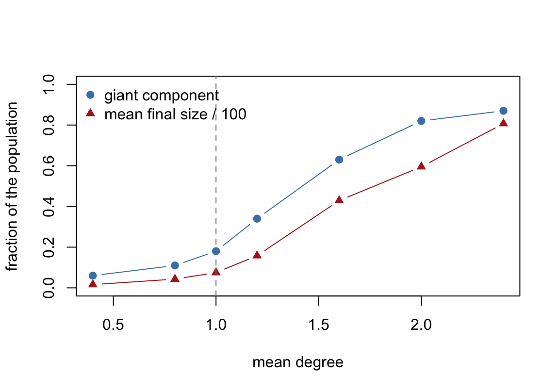
Plotted, the transition is unmistakable. Below mean degree 1 the giant component is a few percent and epidemics fizzle. Around mean degree 1 the giant component lifts off and take-off becomes possible. By mean degree 2 most of the graph is one component and most seeds reach most of it. The final size tracks the giant component because on a frozen graph with certain transmission, a seed infects exactly its own component. It tracks but sits below: a seed reaches the giant component only if it lands there, so the mean final size runs closer to the giant fraction *squared* (roughly, the chance of seeding the giant times its size) than to the giant fraction itself. The two curves rise together and meet only as the giant swallows the whole graph.
```{r threshold-plot, fig.width=6, fig.height=4.2}
plot(sweep$mean_degree, sweep$giant_component, type = "b", pch = 19,
     col = "steelblue", ylim = c(0, 1),
     xlab = "mean degree", ylab = "fraction of the population")
lines(sweep$mean_degree, sweep$mean_final_size / 100, type = "b",
      pch = 17, col = "firebrick")
abline(v = 1, lty = 2, col = "grey50")
legend("topleft", bty = "n", pch = c(19, 17),
       col = c("steelblue", "firebrick"),
       legend = c("giant component", "mean final size / 100"))
```
::: {.callout-note .concept}
## The threshold is a real result, and a slow-network result
The epidemic threshold is one of network epidemiology's central results: a sharp prediction that an epidemic's very possibility turns on a single structural number. But read the assumption under it. It is computed on a fixed graph, and a fixed graph is the slow-network limit, the case where the network never changes during the epidemic. For decades a fixed graph was the only network on which a model could tractably run an epidemic, which is part of why percolation came to feel like *the* fundamental picture. It is fundamental for its regime. In the next section we speed the network up at the identical momentary degree and watch this structural barrier stop binding.
:::
A frozen network is a movie in which only the colors change, never the edges. At mean degree 0.8, below where a giant component has formed, each seed saturates its small cluster in a few steps and then stops. The infection does not slow down; it runs out of network.
```{r frozen-fit, message=FALSE, warning=FALSE, results="hide"}
set.seed(1234)
nw <- network_initialize(100)
est.frozen <- netest(nw, ~edges, 40,
                     dissolution_coefs(~offset(edges), duration = 1e5), verbose = FALSE)
sim.frozen <- netsim(est.frozen, movie.param, movie.init, movie.control)
```
```{r frozen-movie, message=FALSE, fig.width=6}
animate(sim.frozen)
```
## The Fast Limit: Temporal Reachability
Now hold the momentary network fixed and speed the clock up. Same mean degree 0.8 (40 edges), but a duration of 2 instead of frozen. At any instant the network looks identical to the frozen one above, sparse, well below the percolation threshold. Over time it is a different object.
The right question on a dynamic network is not "what component am I in" but "whom can I reach by a **time-respecting path**": a sequence of contacts that moves forward in time, since you cannot infect through a partnership that ended before you were infected. `tsna::tReach()` computes exactly this, returning for each node the size of its forward-reachable set (the node itself plus everyone it can reach by a forward time-respecting path). We compare it to two static baselines: the giant component of a single snapshot, and the giant component of the cumulative graph (the union of every partnership over the window).
```{r fast-limit, message=FALSE, warning=FALSE, results="hide"}
set.seed(1234)
nw <- network_initialize(100)
est.churn <- netest(nw, ~edges, 40,
                    dissolution_coefs(~offset(edges), duration = 2), verbose = FALSE)
dx  <- netdx(est.churn, nsims = 1, nsteps = 50, dynamic = TRUE,
             keep.tnetwork = TRUE, verbose = FALSE)
nwd <- get_network(dx, sim = 1)

snapshot_giant     <- max(component.dist(network.collapse(nwd, at = 25),
                                         connected = "weak")$csize)
temporal_reach     <- mean(tReach(nwd, direction = "fwd"))
cumulative_ceiling <- max(component.dist(network.collapse(nwd, onset = 1, terminus = 51),
                                         connected = "weak")$csize)
```
```{r fast-limit-show}
c(snapshot_giant     = snapshot_giant,
  temporal_reach     = round(temporal_reach),
  cumulative_ceiling = cumulative_ceiling)
```
A single snapshot of this network, the picture percolation theory would work from, holds a giant component of about 8 nodes and predicts no epidemic. But because the network churns, time-respecting paths reach all 100. The snapshot understates the reachable set more than twelvefold. The cumulative graph, the union of every partnership over the 50 steps, connects all 100 as well, and here temporal reach hits that ceiling; when the churn is faster or the horizon shorter, time-ordering can hold reach below the ceiling (not everyone in the union is reachable in the right order), but the direction never reverses: dynamism expands reach far past any snapshot.
::: {.callout-note .concept}
## Same momentary degree, opposite reach: the percolation threshold is a slow-network property
The frozen network and this churning one draw their momentary structure from the **same** subcritical ensemble: mean degree 0.8, a giant component of only about a tenth of the population (the snapshot above found 8 of 100). On the frozen network the epidemic dies inside that little component. On the churning one, with the identical sparse snapshot, time-respecting paths reach the whole population. The only thing that differs is the network clock. So the *percolation* threshold, the connectivity barrier that looks like a fixed feature of a mean degree, is really a feature of the slow-network limit: speed the network up and it stops binding.
Be precise about the scope, though. What stops binding here is the *structural* threshold, connectivity, and it stops binding because we transmit with certainty on a network with no recovery, so connectivity is the only possible barrier to spread. A disease with finite transmissibility and recovery does not lose its threshold when the network speeds up; in the fast limit it meets the classic mass-action $R_0$ threshold instead. The lesson is narrower and sharper than "fast networks have no threshold": the *percolation* threshold is one regime of a larger picture, the slow-network one, that dynamic network models can represent.
:::
The movie makes the contrast plain. Same mean degree as the frozen run, same sparse snapshot, but now the edges churn, and the infection never runs out of network.
```{r churn-fit, message=FALSE, warning=FALSE, results="hide"}
sim.churn <- netsim(est.churn, movie.param, movie.init, movie.control)
```
```{r churn-movie, message=FALSE, fig.width=6}
animate(sim.churn)
```
## The Two Regimes, and Where Concurrency Fits
Put the two limits side by side as the two ends of the clock ratio:
| network clock vs epidemic clock | regime | what governs reach | momentary vs cumulative degree |
|---|---|---|---|
| network much **slower** | frozen / percolation | the static component (structure) | identical |
| network much **faster** | rapid mixing / mass action | the cumulative contact set (timing) | wildly different |
Where does concurrency fit? Not as a third thing beside the two limits, but as a mechanism inside the dynamic regime, and a precise one. A churning network reaches past its snapshot because time-respecting paths keep opening, and concurrency is one way they open. Serial monogamy makes an infection wait: you cannot pass it to a second partner until the first tie ends and the next forms, so the time-ordering of ties throttles forward reach. Overlapping partnerships remove that wait, letting the infection move to a second partner while the first tie is still active. Concurrency, then, raises temporal reachability by relaxing the time-ordering of a dynamic network, which is why, back in the duration tutorial, removing concurrency lowered the final size even at a fixed partnership duration: serial monogamy is not less connected on paper, it is less connected *in time*.
That framing also fixes a trap. Concurrency is a property of the *dynamic* network, not the frozen one. A frozen graph is maximally concurrent by construction (every tie coexists with every other, as the [duration tutorial](mod5-Timing.html) noted), and yet its epidemic dies at mean degree 0.8, because nothing ever turns over: overlap with no churn is inert. Concurrency does its work only while ties are forming and dissolving, which is why it belongs to the fast-clock regime and not to the frozen limit that happens to maximize it.
Two things then explain why concurrency, rather than percolation, became the field's keystone, and both are about its subject matter. The first is timescale: the diseases that drove the concurrency literature, HIV above all, are slow epidemics, generations measured in months or years, on sexual networks that turn over faster than that, so the dynamic regime, where the time-ordering of ties is decisive, is the relevant one.
The second is **density**. Sexual networks are inherently sparse, mean degree rarely exceeds one, which puts their momentary structure at or below the static percolation threshold, where a frozen graph carries no epidemic at all. On such a network the static structure alone cannot spread the infection, so everything rides on the dynamic reachability the ties provide over time, and there the contrast between concurrent and sequential ties is sharpest: a non-linear tipping point in the sub-threshold range where percolation alone predicts nothing. Respiratory contact networks sit in the opposite corner. Contacts are more transient, a faster network clock than sexual ties, but far denser, since social contact rates dwarf sexual ones, so mean degree runs well above one and the momentary network already clears the structural threshold. There the static, percolation lens is the natural one, which is why degree and components, not concurrency, dominate the respiratory conversation.
Neither lens is more fundamental than the other; each is the right tool for one corner of a two-question space. The transferable skill this appendix leaves you with is to ask those two questions first: how fast does the network turn over, relative to how fast the epidemic moves, and how dense is it relative to the percolation threshold? The answers tell you whether the static structure or its dynamics will govern the epidemic, before you commit to a percolation model or a concurrency one. Matching the lens to the clock and the density, rather than the reverse, is the habit worth carrying out of this module and into your own models.