flowchart LR
    S["<b>S</b><br/>Susceptible"] -->|"infection<br/>(se.flow)"| E["<b>E</b><br/>Latent"]

    E -->|"clinical: prop.clinical<br/>eip.rate"| Ip["<b>Ip</b><br/>Pre-symptomatic"]
    E -->|"sub-clinical: 1 - prop.clinical<br/>ea.rate"| A["<b>A</b><br/>Asymptomatic"]

    Ip -->|"ipic.rate"| Ic["<b>Ic</b><br/>Symptomatic"]
    Ic -->|"icr.rate"| R["<b>R</b><br/>Recovered"]
    A -->|"ar.rate"| R

    Ic -.->|"disease<br/>mortality"| Death(( ))

    Ic -.->|"dx.rate.sympt"| DX{{"Diagnosed +<br/>(dxStatus = 2)"}}
    Ip -.->|"dx.rate.other"| DX
    A -.->|"dx.rate.other"| DX
    DX -.->|"case isolation"| ISO["reduced act.rate<br/>(act.rate.dx.inter.rr)"]

    style S fill:#3498db,color:#fff
    style E fill:#8e44ad,color:#fff
    style A fill:#16a085,color:#fff
    style Ip fill:#f39c12,color:#fff
    style Ic fill:#e74c3c,color:#fff
    style R fill:#27ae60,color:#fff
    style DX fill:#34495e,color:#fff
    style ISO fill:#7f8c8d,color:#fff
    style Death fill:none,stroke:none
60 COVID Asymptomatic Infections and Screening
In this tutorial, we will build on our COVID model by adding a more complex disease progression structure, with clinical versus sub-clinical (asymptomatic) pathways, as well as disease screening and diagnosis-based interventions.
Note
This tutorial has two R scripts you should download: a primary script containing the code below and a separate module script. Download both and put them in the same working directory.
60.1 Model Structure
Chapter 58 tracked a single infectious compartment. Here we split infection into two pathways that diverge as people leave the latent state E: a clinical (symptomatic) pathway through a pre-symptomatic stage Ip and a symptomatic stage Ic, and a sub-clinical (asymptomatic) pathway A. Each person’s pathway is drawn once, from an age-specific probability prop.clinical, and fixed for the rest of their infection. Running alongside the disease process, a screening module diagnoses cases (at a higher rate when symptomatic) and, optionally, triggers case isolation for those who test positive.
Solid arrows are disease-state transitions; dashed arrows are the mortality, screening, and isolation processes layered on top.
New parameters, added on top of Chapter 58. The single-rate SEIR progression (ei.rate, ir.rate) is replaced by the six pathway-specific rates below, and new parameters govern relative asymptomatic infectiousness, screening, and case isolation. All rates are per-day probabilities, expressed as the reciprocal of the mean days in the current stage.
| Category | Parameter | Role in the model | Value here |
|---|---|---|---|
| Disease progression | prop.clinical |
Probability of entering the clinical (vs. sub-clinical) pathway on leaving E, as a vector by age decade |
c(0.40, 0.25, 0.37, 0.42, 0.51, 0.59, 0.72, 0.76) |
eip.rate |
E to Ip rate, clinical pathway |
1/4.0 |
|
ipic.rate |
Ip to Ic rate |
1/1.5 |
|
icr.rate |
Ic to R recovery rate |
1/3.5 |
|
ea.rate |
E to A rate, sub-clinical pathway |
1/4.0 |
|
ar.rate |
A to R recovery rate |
1/5.0 |
|
| Transmission | inf.prob.a.rr |
Relative infectiousness of asymptomatic (A) nodes vs. the clinical infectious states |
0.5 |
| Screening and diagnosis | dx.rate.sympt |
Per-step probability of testing while symptomatic (Ic) |
0.2 |
dx.rate.other |
Per-step probability of testing in any other state | 0.01 |
|
pcr.sens |
PCR sensitivity, so 1 - pcr.sens is the false-negative probability |
0.8 |
|
allow.rescreen |
Whether a test-negative person can be tested again | FALSE |
|
| Case isolation | act.rate.dx.inter.time |
Step at which isolation of diagnosed-positive nodes begins | Inf (off) |
act.rate.dx.inter.rr |
Relative act rate for diagnosed-positive nodes once isolation is active | 0.05 |
New model features. Beyond the parameters, this step adds disease states, nodal attributes, a new module, and new summary outputs.
| Feature | What is new relative to Chapter 58 |
|---|---|
| Disease states | The single infectious I becomes three states: pre-symptomatic Ip, symptomatic Ic, and asymptomatic A |
| Nodal attributes | Adds statusTime (step of the last state change, which blocks multi-state jumps in one step), clinical (pathway indicator), and dxStatus (0 never tested, 1 test-negative, 2 test-positive) |
| New module | dx_covid, a screening and diagnosis module with symptomatic and asymptomatic testing streams and imperfect test sensitivity |
| Updated modules | progress2 (two-pathway progression), infect2 (three infectious states of differing infectiousness, plus diagnosis-triggered isolation), and afunc2 / dfunc2 (initialize and track the new attributes) |
| New outputs | Stage flows (ea.flow, ar.flow, eip.flow, ipic.flow, icr.flow) and state sizes (a.num, ip.num, ic.num, e.num, r.num), plus diagnosis counts (nDx, nDx.pos, nDx.pos.sympt, nDx.pos.fn) |
60.2 Setup
First start by loading EpiModel and clearing your global environment.
We will use the network model parameterization and extension functions from the previous tutorial as the starting point for this tutorial.
60.3 Network Initialization
The network will have the same age and aging structure as the previous model. We have to reinitialize the mortality rates as in the last model.
The network size and age attribute are next added.
We will also initialize the status vector as in the past model, plus add three new nodal attributes that are needed for the new extension epidemic models. statusTime will track when a node changes disease stage; it is initialized as NA for everyone and then set to time step 1 for those who are infected. clinical will be a binary attribute to record whether nodes are in a clinical or subclinical pathway; this will be initialized as NA for everyone because it is updated at the move of transition out of the latent (E) state. Finally, dxStatus will keep track of the diagnosed nodal status; it will have three values (0 for never screened, 1 for screened negative, and 2 for screened positive), but everyone will be initialized as 0. As with the others, all nodal attributes are set on the network object with set_vertex_attribute.
Code
statusVec <- rep("s", n)
init.latent <- sample(1:n, 50)
statusVec[init.latent] <- "e"

statusTime <- rep(NA, n)
statusTime[which(statusVec == "e")] <- 1

clinical <- rep(NA, n)
dxStatus <- rep(0, n)

nw <- set_vertex_attribute(nw, "status", statusVec)
nw <- set_vertex_attribute(nw, "statusTime", statusTime)
nw <- set_vertex_attribute(nw, "clinical", clinical)
nw <- set_vertex_attribute(nw, "dxStatus", dxStatus)
nw
Network attributes:
vertices = 1000
directed = FALSE
hyper = FALSE
loops = FALSE
multiple = FALSE
bipartite = FALSE
total edges= 0
missing edges= 0
non-missing edges= 0
Vertex attribute names:
age clinical dxStatus status statusTime vertex.names
No edge attributes60.4 New Modules
The new epidemic modules will involve some minor and major updates to our extension modules from the previous tutorial, and the addition of a new module to handle COVID screening and diagnosis.
60.4.1 Progression
The more sophisticated progression module that we develop below extends the SEIR diagram. Persons who are infected enter one of two pathways: a clinical (symptomatic) pathway and a sub-clinical (asymptomatic) pathway. This follows emerging research suggesting that a substantial fraction of COVID cases never experience any symptoms yet still transmit (although likely at a lower rate). In the clinical pathway, persons are further subdivided into a pre-symptomatic and symptomatic phase to reflect that infectiousness may occur just prior to symptoms.
In the updated progression function below, we build out in code the pathways just described. Each transition from one state to another involves a random Bernoulli process with the probability equal to the transition rate (which is the reciprocal of the average time spent in the current state before transition).
To determine how people enter the subclinical versus clinical pathway, we will use the prop.clinical parameter, which is actually a vector of probabilities corresponding to decade of age. This will allow the level of asymptomatic infection to decrease over age, as evidence suggests. The age.group calculation involves rounding down the continous age in years to a decade, which is then used to index the prop.clinical vector. The clinical attribute is then assigned and stays with each person throughout their infection.
Note that we also include a feature here of tracking the individual statusTime, which is the time step of transition from one state to another. This allows us to prevent immediate transitions across multiple states within a single time step, since the condition for transition requires statusTime < at.
Code
progress2 <- function(dat, at) {

  ## Attributes
  active <- get_attr(dat, "active")
  status <- get_attr(dat, "status")
  age <- get_attr(dat, "age")
  statusTime <- get_attr(dat, "statusTime")
  clinical <- get_attr(dat, "clinical")

  ## Parameters
  prop.clinical <- get_param(dat, "prop.clinical")
  ea.rate <- get_param(dat, "ea.rate")
  ar.rate <- get_param(dat, "ar.rate")
  eip.rate <- get_param(dat, "eip.rate")
  ipic.rate <- get_param(dat, "ipic.rate")
  icr.rate <- get_param(dat, "icr.rate")

  ## Determine Subclinical (E to A) or Clinical (E to Ip to Ic) pathway
  ids.newInf <- which(active == 1 & status == "e" & statusTime <= at & is.na(clinical))
  num.newInf <- length(ids.newInf)
  if (num.newInf > 0) {
    age.group <- pmin((floor(age[ids.newInf] / 10)) + 1, 8)
    prop.clin.vec <- prop.clinical[age.group]
    if (any(is.na(prop.clin.vec))) stop("error in prop.clin.vec")
    vec.new.clinical <- rbinom(num.newInf, 1, prop.clin.vec)
    clinical[ids.newInf] <- vec.new.clinical
  }

  ## Subclinical Pathway
  # E to A: latent move to asymptomatic infectious
  num.new.EtoA <- 0
  ids.Es <- which(active == 1 & status == "e" & statusTime < at & clinical == 0)
  num.Es <- length(ids.Es)
  if (num.Es > 0) {
    vec.new.A <- which(rbinom(num.Es, 1, ea.rate) == 1)
    if (length(vec.new.A) > 0) {
      ids.new.A <- ids.Es[vec.new.A]
      num.new.EtoA <- length(ids.new.A)
      status[ids.new.A] <- "a"
      statusTime[ids.new.A] <- at
    }
  }

  # A to R: asymptomatic infectious move to recovered
  num.new.AtoR <- 0
  ids.A <- which(active == 1 & status == "a" & statusTime < at & clinical == 0)
  num.A <- length(ids.A)
  if (num.A > 0) {
    vec.new.R <- which(rbinom(num.A, 1, ar.rate) == 1)
    if (length(vec.new.R) > 0) {
      ids.new.R <- ids.A[vec.new.R]
      num.new.AtoR <- length(ids.new.R)
      status[ids.new.R] <- "r"
      statusTime[ids.new.R] <- at
    }
  }

  ## Clinical Pathway
  # E to Ip: latent move to preclinical infectious
  num.new.EtoIp <- 0
  ids.Ec <- which(active == 1 & status == "e" & statusTime < at & clinical == 1)
  num.Ec <- length(ids.Ec)
  if (num.Ec > 0) {
    vec.new.Ip <- which(rbinom(num.Ec, 1, eip.rate) == 1)
    if (length(vec.new.Ip) > 0) {
      ids.new.Ip <- ids.Ec[vec.new.Ip]
      num.new.EtoIp <- length(ids.new.Ip)
      status[ids.new.Ip] <- "ip"
      statusTime[ids.new.Ip] <- at
    }
  }

  # Ip to Ic: preclinical infectious move to clinical infectious
  num.new.IptoIc <- 0
  ids.Ip <- which(active == 1 & status == "ip" & statusTime < at & clinical == 1)
  num.Ip <- length(ids.Ip)
  if (num.Ip > 0) {
    vec.new.Ic <- which(rbinom(num.Ip, 1, ipic.rate) == 1)
    if (length(vec.new.Ic) > 0) {
      ids.new.Ic <- ids.Ip[vec.new.Ic]
      num.new.IptoIc <- length(ids.new.Ic)
      status[ids.new.Ic] <- "ic"
      statusTime[ids.new.Ic] <- at
    }
  }

  # Ic to R: clinical infectious move to recovered (if not mortality first)
  num.new.IctoR <- 0
  ids.Ic <- which(active == 1 & status == "ic" & statusTime < at & clinical == 1)
  num.Ic <- length(ids.Ic)
  if (num.Ic > 0) {
    vec.new.R <- which(rbinom(num.Ic, 1, icr.rate) == 1)
    if (length(vec.new.R) > 0) {
      ids.new.R <- ids.Ic[vec.new.R]
      num.new.IctoR <- length(ids.new.R)
      status[ids.new.R] <- "r"
      statusTime[ids.new.R] <- at
    }
  }

  ## Save updated status attribute
  dat <- set_attr(dat, "status", status)
  dat <- set_attr(dat, "statusTime", statusTime)
  dat <- set_attr(dat, "clinical", clinical)

  ## Save summary statistics
  dat <- set_epi(dat, "ea.flow", at, num.new.EtoA)
  dat <- set_epi(dat, "ar.flow", at, num.new.AtoR)
  dat <- set_epi(dat, "eip.flow", at, num.new.EtoIp)
  dat <- set_epi(dat, "ipic.flow", at, num.new.IptoIc)
  dat <- set_epi(dat, "icr.flow", at, num.new.IctoR)

  dat <- set_epi(dat, "e.num", at, sum(status == "e"))
  dat <- set_epi(dat, "a.num", at, sum(status == "a"))
  dat <- set_epi(dat, "ip.num", at, sum(status == "ip"))
  dat <- set_epi(dat, "ic.num", at, sum(status == "ic"))
  dat <- set_epi(dat, "r.num", at, sum(status == "r"))

  return(dat)
}
At the end of the function, we reset the relevant attributes that have changed on the dat object and keep track of all the flow sizes and state sizes. There are several more flows and states to track now, compared to the earlier SEIR model!
60.4.2 Diagnosis
The diagnosis module will handle the process for screening of cases, which here is controlled by two screening rate parameters, dx.rate.sympt and dx.rate.other. The former parameter controls the rate of screening for persons currently with symptomatic infection (that is, in the ic disease state), while the latter parameter controls the rate for all other persons. This reflects the higher rates of symptoms-based diagnosis of active cases.
Additionally, we have a logical parameter, allow.rescreen, that controls whether persons who have previously had a negative COVID test can subsequently retest (this is why we wanted to track dxStatus as a three-level variables of never-tested, tested-negative, and tested-positive). Finally, because COVID diagnostics are imperfect, we incorporate PCR sensitive parameter, pcr.sens, to simulate the process of false-negative test results.
Code
dx_covid <- function(dat, at) {

  ## Pull attributes
  active <- get_attr(dat, "active")
  status <- get_attr(dat, "status")
  dxStatus <- get_attr(dat, "dxStatus")

  ## Pull parameters
  dx.rate.sympt <- get_param(dat, "dx.rate.sympt")
  dx.rate.other <- get_param(dat, "dx.rate.other")
  allow.rescreen <- get_param(dat, "allow.rescreen")
  pcr.sens <- get_param(dat, "pcr.sens")

  ## Initialize trackers
  idsDx.sympt <- idsDx.other <- NULL
  idsDx.sympt.pos <- idsDx.other.pos.true <- NULL
  idsDx.sympt.neg <- idsDx.other.pos.false <- NULL

  ## Determine screening eligibility
  idsElig.sympt <- which(active == 1 & dxStatus %in% 0:1 & status == "ic")
  if (allow.rescreen == TRUE) {
    idsElig.other <- which(active == 1 & dxStatus %in% 0:1 &
                             status %in% c("s", "e", "a", "ip", "r"))
  } else {
    idsElig.other <- which(active == 1 & dxStatus == 0 &
                             status %in% c("s", "e", "a", "ip", "r"))
  }

  ## Symptomatic testing
  nElig.sympt <- length(idsElig.sympt)
  if (nElig.sympt > 0) {
    vecDx.sympt <- which(rbinom(nElig.sympt, 1, dx.rate.sympt) == 1)
    idsDx.sympt <- idsElig.sympt[vecDx.sympt]
    nDx.sympt <- length(idsDx.sympt)
    if (nDx.sympt > 0) {
      vecDx.sympt.pos <- rbinom(nDx.sympt, 1, pcr.sens)
      idsDx.sympt.pos <- idsDx.sympt[which(vecDx.sympt.pos == 1)]
      idsDx.sympt.neg <- idsDx.sympt[which(vecDx.sympt.pos == 0)]
      dxStatus[idsDx.sympt.pos] <- 2
      dxStatus[idsDx.sympt.neg] <- 1
    }
  }

  ## Asymptomatic screening
  nElig.other <- length(idsElig.other)
  if (nElig.other > 0) {
    vecDx.other <- which(rbinom(nElig.other, 1, dx.rate.other) == 1)
    idsDx.other <- idsElig.other[vecDx.other]
    nDx.other <- length(idsDx.other)
    if (nDx.other > 0) {
      idsDx.other.neg <- intersect(idsDx.other, which(status == "s"))
      idsDx.other.pos.all <- intersect(idsDx.other,
                                       which(status %in% c("e", "a", "ip", "r")))
      vecDx.other.pos <- rbinom(length(idsDx.other.pos.all), 1, pcr.sens)
      idsDx.other.pos.true <- idsDx.other.pos.all[which(vecDx.other.pos == 1)]
      idsDx.other.pos.false <- idsDx.other.pos.all[which(vecDx.other.pos == 0)]
      dxStatus[idsDx.other.neg] <- 1
      dxStatus[idsDx.other.pos.false] <- 1
      dxStatus[idsDx.other.pos.true] <- 2
    }
  }

  ## Set attr
  dat <- set_attr(dat, "dxStatus", dxStatus)

  ## Summary statistics
  dat <- set_epi(dat, "nDx", at, length(idsDx.sympt) + length(idsDx.other))
  dat <- set_epi(dat, "nDx.pos", at, length(idsDx.sympt.pos) +
                   length(idsDx.other.pos.true))
  dat <- set_epi(dat, "nDx.pos.sympt", at, length(idsDx.sympt.pos))
  dat <- set_epi(dat, "nDx.pos.fn", at, length(idsDx.sympt.neg) +
                   length(idsDx.other.pos.false))

  return(dat)
}
At the end of the function, we updated the modified dxStatus attribute, and calculate some summary statistics for new cases.
60.4.3 Infection
It is also necessary to update the infection module function in a couple of ways. The first will reflect that we now have 3 infectious disease states, of varying infectiousness, compared to the earlier SEIR model’s one infectious state. This requires modifying the code querying the definition of infectious nodes, and the construction of the discordant edgelist.
Second, onto the discordant edgelist data frame, we add the disease state of the infectious node and the diagnostic status of that node. Those new data are then used in two ways. First, being in the asymptomatic disease state, a, is associated with a lower probability of transmission compared to the other two (clinical) infectious disease states. That is accomplished by modifying the base transmission probability by a relative risk parameter, inf.prob.a.rr.
Second, being infectious and diagnosed positive (which a dxStatus of 2), may trigger behavioral interventions reflect case isolation. This type of behavioral change may be accomplished in several different ways. Here it involves a modification of the act.rate parameter that controls the number of individual exposure events between active dyads in the current time step. This type of intervention may start at a particular time step, act.rate.dx.inter.time, and result in a relative reduction in the current act rate of act.rate.dx.inter.rr.
Code
infect2 <- function(dat, at) {

  ## Uncomment this to run environment interactively
  # browser()

  ## Attributes ##
  active <- get_attr(dat, "active")
  status <- get_attr(dat, "status")
  infTime <- get_attr(dat, "infTime")
  dxStatus <- get_attr(dat, "dxStatus")
  statusTime <- get_attr(dat, "statusTime")

  ## Parameters ##
  inf.prob <- get_param(dat, "inf.prob")
  act.rate <- get_param(dat, "act.rate")
  inf.prob.a.rr <- get_param(dat, "inf.prob.a.rr")
  act.rate.dx.inter.time <- get_param(dat, "act.rate.dx.inter.time")
  act.rate.dx.inter.rr <- get_param(dat, "act.rate.dx.inter.rr")

  ## Find infected nodes ##
  infstat <- c("a", "ic", "ip")
  idsInf <- which(active == 1 & status %in% infstat)
  nActive <- sum(active == 1)
  nElig <- length(idsInf)

  ## Initialize default incidence at 0 ##
  nInf <- 0

  ## If any infected nodes, proceed with transmission ##
  if (nElig > 0 && nElig < nActive) {

    ## Look up discordant edgelist ##
    del <- discord_edgelist(dat, at, infstat = infstat)

    ## If any discordant pairs, proceed ##
    if (!(is.null(del))) {

      del$status <- status[del$inf]
      del$dxStatus <- dxStatus[del$inf]

      # Set parameters on discordant edgelist data frame
      del$transProb <- inf.prob
      del$transProb[del$status == "a"] <- del$transProb[del$status == "a"] *
                                          inf.prob.a.rr
      del$actRate <- act.rate
      if (at >= act.rate.dx.inter.time) {
        del$actRate[del$dxStatus == 2] <- del$actRate[del$dxStatus == 2] *
                                          act.rate.dx.inter.rr
      }
      del$finalProb <- 1 - (1 - del$transProb)^del$actRate

      # Stochastic transmission process
      transmit <- rbinom(nrow(del), 1, del$finalProb)

      # Keep rows where transmission occurred
      del <- del[which(transmit == 1), ]

      # Look up new ids if any transmissions occurred
      idsNewInf <- unique(del$sus)
      nInf <- length(idsNewInf)

      # Set new attributes and transmission matrix
      if (nInf > 0) {
        status[idsNewInf] <- "e"
        infTime[idsNewInf] <- at
        statusTime[idsNewInf] <- at
        dat <- set_transmat(dat, del, at)
      }
    }
  }

  dat <- set_attr(dat, "status", status)
  dat <- set_attr(dat, "infTime", infTime)
  dat <- set_attr(dat, "statusTime", statusTime)

  ## Save summary statistics
  dat <- set_epi(dat, "se.flow", at, nInf)

  return(dat)
}
There are no other modifications of the infection module other than to track the statusTime upon infection and then resetting that attribute on the dat object.
60.4.4 Births
The birth module requires a very minor change to update the three new nodal attributes on the dat object for any incoming nodes.
Code
afunc2 <- function(dat, at) {

  ## Parameters ##
  n <- get_epi(dat, "num", at - 1)
  a.rate <- get_param(dat, "arrival.rate")

  ## Process ##
  nArrivalsExp <- n * a.rate
  nArrivals <- rpois(1, nArrivalsExp)

  # Update attributes
  if (nArrivals > 0) {
    dat <- append_core_attr(dat, at = at, n.new = nArrivals)
    dat <- append_attr(dat, "status", "s", nArrivals)
    dat <- append_attr(dat, "infTime", NA, nArrivals)

    dat <- append_attr(dat, "age", 0, nArrivals)
    dat <- append_attr(dat, "statusTime", NA, nArrivals)
    dat <- append_attr(dat, "clinical", NA, nArrivals)
    dat <- append_attr(dat, "dxStatus", 0, nArrivals)
  }

  ## Summary statistics ##
  dat <- set_epi(dat, "a.flow", at, nArrivals)

  return(dat)
}
60.4.5 Deaths
The death module requires an even more minor modification from the last tutorial, which involves simulating COVID-related mortality and tracking the number of covid.deaths based on deaths that occurs within the ic (clinical symptomatic) state (previously these were in the i state only).
Code
dfunc2 <- function(dat, at) {

  ## Attributes
  active <- get_attr(dat, "active")
  exitTime <- get_attr(dat, "exitTime")
  age <- get_attr(dat, "age")
  status <- get_attr(dat, "status")

  ## Parameters
  dep.rates <- get_param(dat, "departure.rates")
  dep.dis.mult <- get_param(dat, "departure.disease.mult")

  ## Query alive
  idsElig <- which(active == 1)
  nElig <- length(idsElig)

  ## Initialize trackers
  nDepts <- 0
  idsDepts <- NULL

  if (nElig > 0) {

    ## Calculate age-specific departure rates for each eligible node ##
    ## Everyone older than 85 gets the final mortality rate
    whole_ages_of_elig <- pmin(ceiling(age[idsElig]), 86)
    departure_rates_of_elig <- dep.rates[whole_ages_of_elig]

    ## Multiply departure rates for diseased persons
    idsElig.inf <- which(status[idsElig] == "ic")
    departure_rates_of_elig[idsElig.inf] <- departure_rates_of_elig[idsElig.inf] * dep.dis.mult

    ## Simulate departure process
    vecDepts <- which(rbinom(nElig, 1, departure_rates_of_elig) == 1)
    idsDepts <- idsElig[vecDepts]
    nDepts <- length(idsDepts)

    ## Update nodal attributes
    if (nDepts > 0) {
      active[idsDepts] <- 0
      exitTime[idsDepts] <- at
    }
  }

  ## Reset attributes
  dat <- set_attr(dat, "active", active)
  dat <- set_attr(dat, "exitTime", exitTime)

  ## Summary statistics ##
  dat <- set_epi(dat, "total.deaths", at, nDepts)

  # covid deaths
  covid.deaths <- length(intersect(idsDepts, which(status == "ic")))
  dat <- set_epi(dat, "covid.deaths", at, covid.deaths)


  return(dat)
}
60.5 Network Model Estimation
With epidemic modules designed, we parameterize the exact same network model as the previous tutorial.
Code
[1] 1000 80 2000Dissolution Coefficients
=======================
Dissolution Model: ~offset(edges)
Target Statistics: 20
Crude Coefficient: 2.944439
Mortality/Exit Rate: 3.159205e-05
Adjusted Coefficient: 2.945703We estimate the model with netest. Here we demonstrate how to increase the maximum number of MCMLE iterations (the default is 20), which was sometimes necessary to get this model to converge.
Model diagnostics look similar to last time.
Code
Network Diagnostics
-----------------------
- Simulating 10 networks
- Calculating formation statisticsEpiModel Network Diagnostics
=======================
Diagnostic Method: Dynamic
Simulations: 10
Time Steps per Sim: 500
Formation Diagnostics
-----------------------
Target Sim Mean Pct Diff Sim SE Z Score SD(Sim Means) SD(Statistic)
edges 1000 983.856 -1.614 1.577 -10.236 8.095 24.656
absdiff.age 2000 1955.853 -2.207 5.311 -8.313 22.660 77.668
degree0 80 89.751 12.188 0.431 22.612 1.243 9.872
degree1 NA 323.191 NA 0.693 NA 4.084 15.619
degree2 NA 292.188 NA 0.601 NA 2.152 14.970
degree3 NA 175.249 NA 0.463 NA 1.867 12.183
degree4 NA 79.181 NA 0.399 NA 1.976 9.308
degree5 NA 28.754 NA 0.186 NA 1.058 5.284
degree6 NA 8.694 NA 0.108 NA 0.609 3.038
Duration Diagnostics
-----------------------
Target Sim Mean Pct Diff Sim SE Z Score SD(Sim Means) SD(Statistic)
edges 20 20.03 0.152 0.057 0.538 0.132 0.651
Dissolution Diagnostics
-----------------------
Target Sim Mean Pct Diff Sim SE Z Score SD(Sim Means) SD(Statistic)
edges 0.05 0.05 -0.018 0 -0.093 0 0.007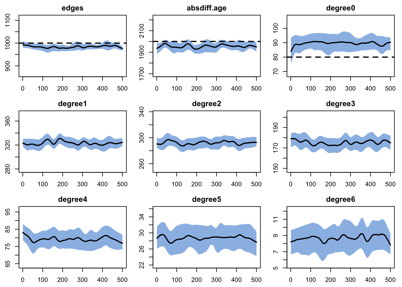
60.6 Epidemic Model Simulation
We are now using more realistic COVID parameters for disease progression, based on the current literature and other models. Note that the current parameters allow for 50% lower transmissibility in the asymptomatic stage, age-varying clinical pathways, a PCR sensitivity of 80%, a diagnosis rate that is 20-fold higher for those with symptomatic infection, and no rescreening. We have also prevented any case isolation by setting the act.rate.dx.inter.time to Inf.
Code
param <- param.net(inf.prob = 0.1,
                   act.rate = 3,
                   departure.rates = dr_vec,
                   departure.disease.mult = 1000,
                   arrival.rate = 1/(365*85),
                   inf.prob.a.rr = 0.5,
                   act.rate.dx.inter.time = Inf,
                   act.rate.dx.inter.rr = 0.05,
                   # proportion in clinical pathway by age decade
                   prop.clinical = c(0.40, 0.25, 0.37, 0.42, 0.51, 0.59, 0.72, 0.76),
                   ea.rate = 1/4.0,
                   ar.rate = 1/5.0,
                   eip.rate = 1/4.0,
                   ipic.rate = 1/1.5,
                   icr.rate = 1/3.5,
                   pcr.sens = 0.8,
                   dx.rate.sympt = 0.2,
                   dx.rate.other = 0.01,
                   allow.rescreen = FALSE)
init <- init.net()
For the control settings, it is necessary to define all the relevant modules for our system, and input the associated functions. We will simulate the model only over 100 days, with 10 simulations. Here we use tergmLite, but this can be set to FALSE to retain the full network data (these simulations will take a bit longer).
Code
source("mod13-COVID2-fx.R")
control <- control.net(type = NULL,
                       nsims = 10,
                       ncores = 5,
                       nsteps = 100,
                       infection.FUN = infect2,
                       progress.FUN = progress2,
                       dx.FUN = dx_covid,
                       aging.FUN = aging,
                       departures.FUN = dfunc2,
                       arrivals.FUN = afunc2,
                       resimulate.network = TRUE,
                       tergmLite = TRUE,
                       set.control.tergm =
                         control.simulate.formula.tergm(MCMC.burnin.min = 10000))
The model is then simulated with netsim.
60.7 Model Analysis
Let’s print out the netsim object to review the available data variables.
EpiModel Simulation
=======================
Model class: netsim

Simulation Summary
-----------------------
Model type:
No. simulations: 10
No. time steps: 100
No. NW groups: 1

Fixed Parameters
---------------------------
inf.prob = 0.1
act.rate = 3
departure.rates = 1.612192e-05 6.794521e-07 6.794521e-07 6.794521e-07
6.794521e-07 3.205479e-07 3.205479e-07 3.205479e-07 3.205479e-07 3.205479e-07
...
departure.disease.mult = 1000
arrival.rate = 3.223207e-05
inf.prob.a.rr = 0.5
act.rate.dx.inter.time = Inf
act.rate.dx.inter.rr = 0.05
prop.clinical = 0.4 0.25 0.37 0.42 0.51 0.59 0.72 0.76
ea.rate = 0.25
ar.rate = 0.2
eip.rate = 0.25
ipic.rate = 0.6666667
icr.rate = 0.2857143
pcr.sens = 0.8
dx.rate.sympt = 0.2
dx.rate.other = 0.01
allow.rescreen = FALSE
groups = 1

Model Functions
-----------------------
initialize.FUN
resim_nets.FUN
summary_nets.FUN
infection.FUN
departures.FUN
arrivals.FUN
nwupdate.FUN
prevalence.FUN
verbose.FUN
progress.FUN
dx.FUN
aging.FUN

Model Output
-----------------------
Variables: s.num i.num num ea.flow ar.flow eip.flow
ipic.flow icr.flow e.num a.num ip.num ic.num r.num nDx
nDx.pos nDx.pos.sympt nDx.pos.fn meanAge se.flow
total.deaths covid.deaths a.flow
Networks: sim1 ... sim10
Transmissions: sim1 ... sim10

Formation Statistics
-----------------------
            Target Sim Mean Pct Diff Sim SE Z Score SD(Sim Means) SD(Statistic)
edges         1000  962.793   -3.721  4.684  -7.943        16.224        33.175
degree0         80   87.140    8.925  0.889   8.028         2.808         9.822
absdiff.age   2000 1935.328   -3.234 13.057  -4.953        40.262        90.501


Duration and Dissolution Statistics
-----------------------
Not available when:
- `control$tergmLite == TRUE`
- `control$save.network == FALSE`
- `control$save.diss.stats == FALSE`
- dissolution formula is not `~ offset(edges)`
- `keep.diss.stats == FALSE` (if merging)
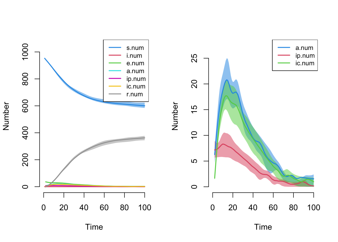
Here is a plot of disease state sizes over time. The default plot makes it difficult to see the prevalence because the susceptible and recovered state sizes are much larger overall, so we plot just the three infectious states alone.
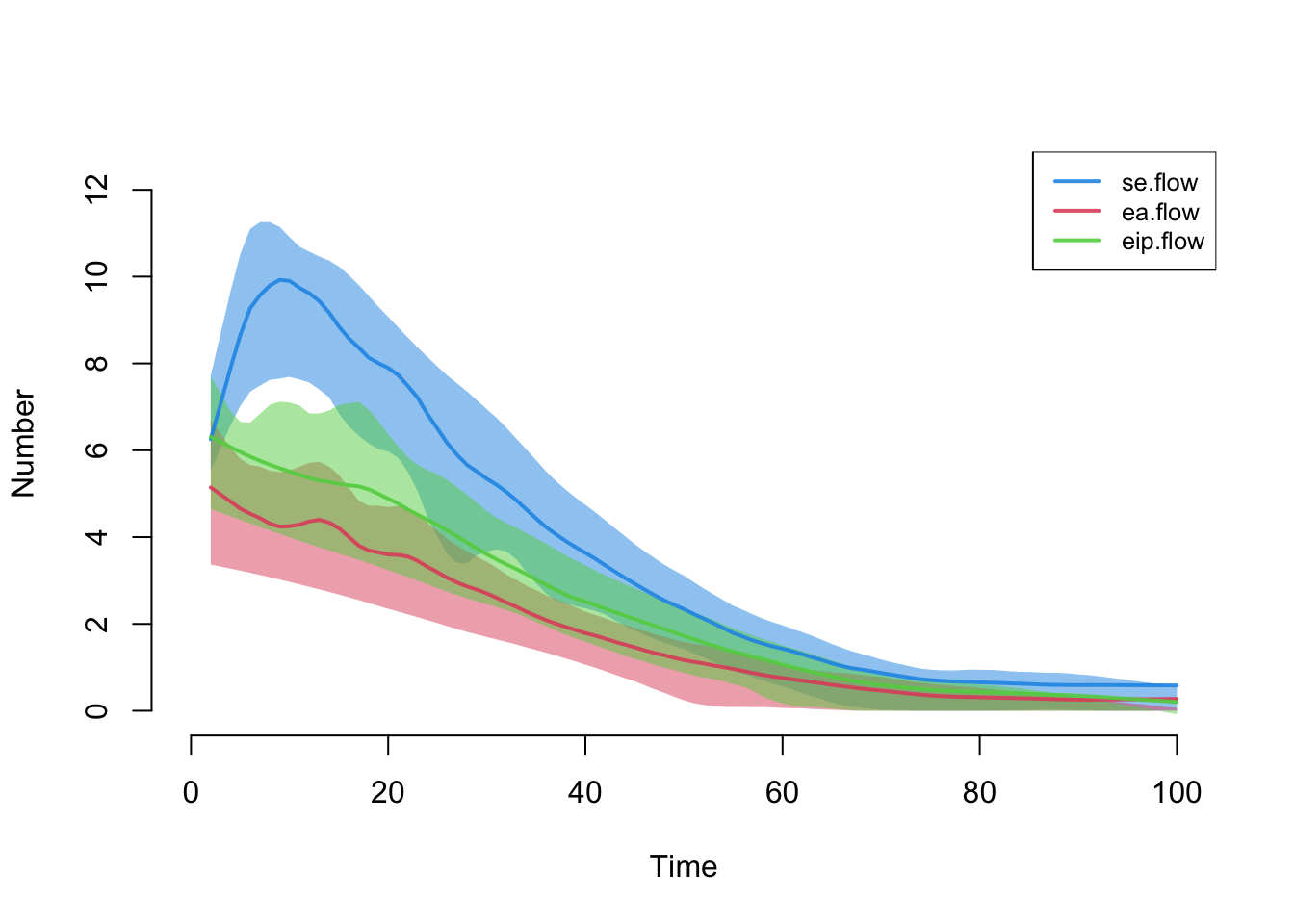
Here are the first three transitions after leaving the suceptible state.
Finally, we can export the mean data, averaged across the 10 simulations.
  time s.num i.num    num ea.flow ar.flow eip.flow ipic.flow icr.flow e.num
1    1 950.0     0 1000.0     NaN     NaN      NaN       NaN      NaN   NaN
2    2 944.1     0  999.9     5.4     0.0      7.3       0.0      0.0  37.3
3    3 936.5     0  999.4     4.8     1.4      5.0       5.2      0.0  33.3
4    4 928.2     0  999.0     4.7     2.2      5.4       4.6      1.1  30.8
5    5 919.8     0  998.6     4.2     2.9      3.9       5.7      2.3  31.2
6    6 908.6     0  997.8     4.4     3.2      6.1       4.0      2.9  29.1
  a.num ip.num ic.num r.num  nDx nDx.pos nDx.pos.sympt nDx.pos.fn  meanAge
1   NaN    NaN    NaN   NaN  NaN     NaN           NaN        NaN      NaN
2   5.4    7.3    0.0   0.0 10.7     0.4           0.0        0.1 42.57174
3   8.8    7.1    5.2   1.4 10.5     1.4           1.0        0.3 42.57023
4  11.3    7.9    8.2   4.7 11.5     1.2           0.8        0.3 42.55251
5  12.6    6.1   11.0   9.9 11.5     2.1           1.8        0.2 42.52304
6  13.8    8.2   11.7  16.0 11.7     2.4           1.7        0.7 42.51405
  se.flow total.deaths covid.deaths a.flow
1     NaN          NaN          NaN    NaN
2     5.8          0.1          0.0    0.0
3     7.6          0.5          0.5    0.0
4     8.5          0.6          0.6    0.2
5     8.4          0.4          0.4    0.0
6    11.2          0.9          0.7    0.1
And calculate the average cumulative incidence.