# Clustering and Heterogeneity
The previous tutorial changed *timing*, how partnerships overlap and how long they last. This one changes *structure*: whether contacts cluster into tight local groups, and whether contact patterns and durations depend on who people are. This is the most involved network we build by hand in these visualization tutorials, so we build it up one term at a time.
::: {.callout-note}
Download the R script to follow along with this tutorial [here](mod5-Structure.R).
:::
## Setup
Same packages, animation helper, and fixed epidemic as the timing tutorial. The `inf.prob = 1` means every contact transmits with certainty, a deliberate extreme so that differences between the movies and the infection counts come from the network structure alone, not from the disease.
```{r setup, message = FALSE, warning=FALSE}
library("EpiModel")
library("ndtv")
library("htmlwidgets")

slice.par  <- list(start = 1, end = 25, interval = 1, aggregate.dur = 1, rule = "any")
render.par <- list(tween.frames = 10, show.time = FALSE)
plot.par   <- list(mar = c(0, 0, 0, 0))

animate <- function(sim, ...) {
  nw <- get_network(sim)
  nw <- color_tea(nw, verbose = FALSE)
  compute.animation(nw, slice.par = slice.par, verbose = FALSE)
  render.d3movie(
    nw, render.par = render.par, plot.par = plot.par,
    vertex.col = "ndtvcol", edge.col = "darkgrey",
    vertex.border = "lightgrey", displaylabels = FALSE,
    output.mode = "htmlWidget", ...)
}

param   <- param.net(inf.prob = 1)
init    <- init.net(i.num = 10)
control <- control.net(type = "SI", nsteps = 25, nsims = 1)
```
## Clustering: Triangles
Clustering means contacts that close **triangles**: if A is tied to B and to C, are B and C also tied to each other? A raw `triangle` term tends to make ERGMs numerically unstable (degenerate), so we use `gwesp`, the geometrically weighted edgewise shared partner term, which is better behaved. We call it `gwesp(0, TRUE)`: the first argument is the decay parameter (set to 0), and `fixed = TRUE` holds it fixed rather than estimating it. With the decay fixed at 0, the statistic simplifies to the number of edges that have at least one shared partner, and each such edge closes at least one triangle.
Better behaved is not unconditionally well behaved: `gwesp` still has a feasible range, and asking for too much clustering at a fixed mean degree pushes back toward the instability we were avoiding. The null value here is under 1, so we target 15 of the 40 edges sitting in a triangle. (As with every target, 15 is an expected value; the realized count fluctuates around it.)
```{r tri-netest, message=FALSE, results="hide", warning=FALSE}
set.seed(1234)
nw <- network_initialize(n = 100)
coef.diss <- dissolution_coefs(dissolution = ~offset(edges), duration = 20)
est.tri   <- netest(nw, ~edges + gwesp(0, TRUE), c(40, 15), coef.diss)
sim.tri   <- netsim(est.tri, param, init, control)
```
```{r tri-movie, message=FALSE, fig.width=6}
animate(sim.tri, vertex.cex = 0.9)
```
Are triangles associated with faster or slower spread? In these specifications, **slower**. A triangle gives you a redundant path: once A infects B, B's tie to C is unlikely to reach anyone new, because C is probably already infected by A. Clustering concentrates transmission opportunities among people who have already been reached, so a contact that could have opened a new part of the network gets spent on someone reachable anyway. The same number of edges does less work.
::: {.callout-note}
## "Slower" is a direction here, not a law about triangles
Clustering slows spread in this setup, and the replicated runs below back that. But whether it does, and by how much, depends on the disease natural history, the rest of the network (degree distribution and degree correlations), the seeding, and which outcome you measure: final size, peak height, or early growth rate can respond differently, and in some regimes clustering can even speed early local growth. Read this as the direction under these specifications, not as a property of triangles in general.
:::
Here is the replicated evidence for the direction, 200 runs each:
```{r tri-evidence, message=FALSE, warning=FALSE, results="hide"}
final_prev <- function(est, nsims = 200) {
  sim <- netsim(est, param, init,
                control.net(type = "SI", nsteps = 25, nsims = nsims,
                            ncores = 5, verbose = FALSE))
  d <- as.data.frame(sim, out = "mean"); round(d$i.num[d$time == 25], 1)
}
set.seed(1234)
nw0 <- network_initialize(n = 100)
est.base <- netest(nw0, ~edges, 40, coef.diss, verbose = FALSE)

tri.evidence <- data.frame(
  specification = c("Baseline (edges only)", "With clustering (gwesp target 15)"),
  mean_infected_of_100 = c(final_prev(est.base), final_prev(est.tri)))
```
```{r tri-evidence-show}
tri.evidence
```
By step 25, the clustered network has reached fewer people on average than the baseline with the same mean degree. Because `inf.prob = 1` eventually saturates whatever the network can reach, this gap is about how *fast* the infection spreads within the 25-step window, not the final size it would reach given unlimited time.
## Heterogeneous Networks: Attributes
So far every node has been interchangeable except for infection status. Now we let contact patterns depend on **who people are**, using two ordinary (non-special) nodal attributes: a binary `community` (think of any geographic, demographic, or social split that shapes who contacts whom) and an integer `age` between 18 and 50.
```{r attr-network}
set.seed(1234)
nw <- network_initialize(n = 100)
nw <- set_vertex_attribute(nw, "community", rbinom(100, 1, 0.5))
nw <- set_vertex_attribute(nw, "age", sample(18:50, 100, TRUE))
```
We build the formation model up one term at a time, so each addition's job is separable:
- **`edges`**, target 50: overall mean degree of 1 (`50 * 2 / 100`). We use a slightly denser network than earlier so the added structure has enough edges to be visible.
- **`nodematch("community")`**, target 40: of the 50 edges, 40 are within-community, so only 10 bridge the two communities. This is the community structure.
- **`nodefactor("community")`**, target 70: lets mean degree differ by community. Its statistic is the summed degree of the non-reference group; `nodefactor` uses the lowest attribute value (`community = 0`) as the reference, so 70 is the total degree of the `community = 1` nodes, giving them more ties than average. This is activity heterogeneity.
- **`absdiff("age")`**, target 100: a mixing term for a continuous attribute. Its statistic is the sum of absolute age differences across the 50 edges, so a target of 100 means partners average 2 years apart, strong age assortativity.
- **`concurrent`**, target 30: nodes with two or more simultaneous partners. At mean degree 1, `ppois(1, 1, lower.tail = FALSE) * 100` is about 26 by chance, so 30 asks for slightly more.
Assembled, with each target supplied **in the same order** as its term (the order is positional and nothing labels it, so we write both out one per line):
```{r attr-formation}
formation <- ~edges + # <1>
nodematch("community") + # <2>
nodefactor("community") + # <3>
absdiff("age") + # <4>
concurrent # <5>
target.stats <- c(50, 40, 70, 100, 30)
```
1. Overall edges (mean degree 1).
2. Within-community edges (community structure).
3. Degree of the `community = 1` nodes (activity heterogeneity).
4. Summed absolute age gap across edges (age assortativity).
5. Concurrent nodes.
For now we keep a single homogeneous duration; the next section makes duration depend on partnership type.
```{r attr-netest, message=FALSE, results="hide", warning=FALSE}
est.attr <- netest(nw, formation, target.stats,
                   dissolution_coefs(~offset(edges), duration = 20))
```
To read the two attributes in the movie, we encode `community` as node shape (a square vs an effectively round polygon) and `age` as node size.
```{r attr-fit, message=FALSE, results="hide"}
sim.attr <- netsim(est.attr, param, init, control)
nw.a <- get_network(sim.attr)
community <- get_vertex_attribute(nw.a, "community")
age       <- get_vertex_attribute(nw.a, "age")
```
```{r attr-movie, message=FALSE, fig.width=6}
animate(sim.attr,
        vertex.sides = ifelse(community == 1, 4, 50),
        vertex.cex   = age / 25)
```
The infection now moves preferentially within a community and among people close in age, because that is where the edges are.
## Heterogeneous Dissolution
Every dissolution model so far has been a single global number: one duration for every edge. Here we let duration depend on the *kind* of partnership. Within-community ties will average 10 steps and cross-community ties 20, so within-community ties are both more common and shorter-lived.
```{r het-diss}
coef.diss.het <- dissolution_coefs(
dissolution = ~offset(edges) + offset(nodematch("community")), # <1>
duration = c(20, 10)) # <2>
```
1. The dissolution formula, which must be dyad-independent. `edges` is the baseline that applies to every edge; `nodematch("community")` adjusts it for edges whose endpoints match.
2. The order is the whole trap. The first duration is the *reference* group, the edges that do **not** match on community. The second is the matched group. Swap them and the model is still valid, just backwards from what you meant, and nothing warns you.
::: {.callout-note .definition}
## The dissolution model is a leading subset of the formation model
The two dissolution terms here, `edges` and `nodematch("community")`, are exactly the **first two terms of the formation model, in the same order**. That is required, not incidental. `dissolution_coefs` computes one correction per dissolution term (`coef.form.corr`), and `netest` subtracts each correction from the *positionally corresponding* formation coefficient. So the dissolution formula has to be a leading prefix of the formation formula: same terms, same order, at the start. (This is the current EpiModel convention; the underlying `ergm`/`tergm` machinery has been reworked over recent releases, so if you use an unfamiliar version, confirm against `?dissolution_coefs`.)
:::
::: {.callout-note .concept}
## Why heterogeneous dissolution is harder to read than to write
Specifying this model is easy: you name a duration per partnership type, and the two numbers are independent, 20 means 20 and 10 means 10. Reading it back is where it gets hard, because what the model *stores* is not what you *supplied*.
The coefficients are on the logit scale of *persistence*, where `p = 1 - 1/duration`. The first coefficient is the reference group's persistence logit, `logit(1 - 1/20) = 2.944`, identical to the homogeneous `duration = 20` model. But the second number is **not** the coefficient for a 10-step tie. It is the *increment* added to the baseline for matched edges: the matched persistence logit is `logit(1 - 1/10) = 2.197`, and the stored value is `2.197 - 2.944 = -0.747`. Three things follow:
- **You cannot read a coefficient without knowing the reference group.** `-0.747` means nothing on its own.
- **The sign of the increment is direction, not duration.** Negative means the matched group's ties are shorter than the reference's.
- **Equal durations give an increment of exactly zero**, the homogeneous model reappearing as a special case.
:::
::: {.callout-note .definition}
## What can and cannot vary
Dissolution heterogeneity has to be a property of an **edge**, not a **node**. `nodematch` asks "are these two the same?" and `nodemix` asks "which cell of the mixing matrix does this pair fall in?" Both are questions about the *dyad*, so every edge has exactly one answer and therefore one duration. `nodefactor` is a question about a *node*, and an edge has two of them: an edge between a 20-year-old and a 50-year-old has no single age-group duration without inventing a rule. So `nodematch` and `nodemix` are supported for dissolution and `nodefactor` is not, even though it is perfectly dyad-independent. NME-II's multi-layer models take the other route, giving each relationship type its own network with its own dissolution model.
:::
Now we fit the full model and, crucially, check the durations came out where we asked. This is the only way to *see* the heterogeneity rather than assert it.
```{r het-netest, message=FALSE, results="hide", warning=FALSE}
est.het <- netest(nw, formation, target.stats, coef.diss.het)
```
```{r het-netdx, message=FALSE}
dx <- netdx(est.het, nsims = 5, nsteps = 500, ncores = 5, verbose = FALSE)
dx
```
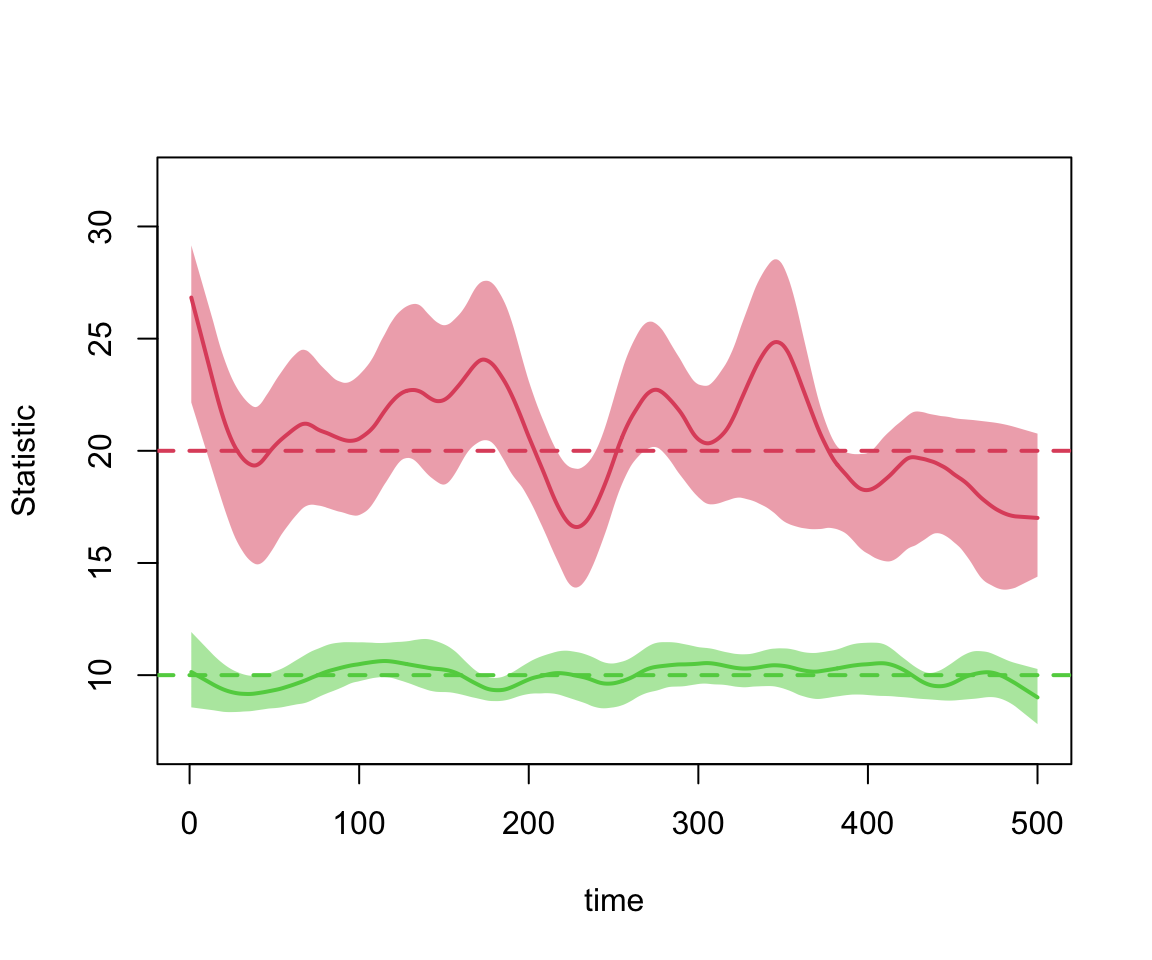
The Duration Diagnostics report the two groups on their natural scale, in time steps: the `edges` row is the reference (non-matched) duration and the `nodematch.community` row is the matched one. They land close to the 20 and 10 we asked for.
::: {.callout-note}
## Two dissolution terms, two corrected formation coefficients
It is a common shorthand, and one earlier version of this tutorial used, that the edges dissolution approximation "corrects only the `edges` coefficient." That is true only for a homogeneous dissolution model. Here the dissolution model has **two** terms, so `netest` corrects **both** corresponding formation coefficients: `edges` and `nodematch("community")`. You can see it by comparing `est.het$coef.form.crude` (the cross-sectional fit) with `est.het$coef.form` (the corrected coefficients the simulation uses): the first two entries differ, and the rest are untouched. That coefficient correction is exact for these dyad-independent terms. The realized dynamic statistics are a separate matter: because the edges dissolution approximation is only a first-order approximation, every formation statistic sits a few percent below its target in dynamic simulation (in the Formation Diagnostics above, all five are 5 to 8 percent under). The dyad-**dependent** `concurrent` term is the one the correction does not fully reach, so it drifts the most, about 8 percent here; that bias grows as durations get shorter, which is a reason not to pick durations shorter than the science requires.
:::
```{r het-durplot, message=FALSE, fig.width=6}
plot(dx, type = "duration")
```
Finally, the movie, with community and age encoded as before.
```{r het-fit, message=FALSE, results="hide"}
sim.het <- netsim(est.het, param, init, control)
nw.h <- get_network(sim.het)
community <- get_vertex_attribute(nw.h, "community")
age       <- get_vertex_attribute(nw.h, "age")
```
```{r het-movie, message=FALSE, fig.width=6}
animate(sim.het,
        vertex.sides = ifelse(community == 1, 4, 50),
        vertex.cex   = age / 25)
```
## Takeaways
- **Clustering** (triangles, via `gwesp`) slows spread in these specifications, because triangles create redundant paths to people already reached. Whether it does in general depends on the disease, the network, the seeding, and the outcome.
- **Nodal attributes** let contact patterns depend on who people are, steering which subgroups the infection reaches.
- **Heterogeneous dissolution** lets partnership duration depend on the kind of partnership, and it is the one place in the course where dissolution is not a single global number. Reading its coefficients requires knowing the reference group, and its dissolution formula must be a leading subset of the formation formula.
Where do all these numbers come from? Every one was chosen, not measured. That is fine for demonstrating a mechanism, which is all this module set out to do, but it is exactly the wrong basis for a research model; the modules that follow are about estimating formation targets and durations from real network data. First, the [lab](mod5-Lab.html) gives you a chance to change one thing at a time and predict what the movie will do. (For anyone who wants to go further, an [optional appendix](mod5-Timescale.html) after the lab develops the timing ideas into a single organizing question: how fast the network turns over, relative to the epidemic.)