53 Appendix: Choosing the Number of Simulations
Every netsim() run is stochastic: the same model, run again, gives a slightly different epidemic. We therefore run many replicates (the nsims argument in control.net()) and summarize across them. This raises a question that comes up in almost every project, and one we are asked often: how many replicates are enough? Too few and the summary is noisy, so an apparent difference between two scenarios may be simulation noise rather than a real effect. Too many and we waste compute, which matters once a design has hundreds of scenarios running on a cluster.
This chapter gives a concrete, defensible way to answer it.
53.1 Monte Carlo error
The mean of an outcome across nsims replicates estimates the model’s expected value for that outcome. Like any sample mean, it carries a Monte Carlo standard error that shrinks with the number of replicates:
\[\text{SE} = \frac{\text{SD}}{\sqrt{n_\text{sims}}}\]
where SD is the standard deviation of the outcome across replicates. The standard error falls only with the square root of nsims, so halving it takes four times as many runs.
The standard error is in the units of the outcome, which makes it awkward to compare across outcomes measured on different scales: a prevalence count, an incidence rate, a number of deaths. The coefficient of variation (CV) rescales it into a unitless fraction of the estimate itself:
\[\text{CV} = \frac{\text{SE}}{\lvert\text{mean}\rvert} = \frac{\text{SD}}{\lvert\text{mean}\rvert \, \sqrt{n_\text{sims}}}\]
In words, the CV is the Monte Carlo noise in the estimate expressed as a fraction of the estimate. A CV of 1% means that if you re-ran the whole pilot, the mean would typically land within about one percent of the value you got; a CV of 20% means it could easily move by a fifth. Because it is scale-free, a single CV target works for every outcome at once, whatever its units, which is exactly what you want when a model reports many different quantities.
That scale-free form is also what makes the CV a sizing tool. Setting it equal to a target and solving for the count gives
\[n_\text{sims} \approx \left(\frac{\text{SD}}{\lvert\text{mean}\rvert \cdot \text{CV}_\text{target}}\right)^{2},\]
so an outcome’s required number of simulations is governed by its relative spread, the SD-to-mean ratio. An outcome with a large mean and modest spread reaches a tight CV in a handful of runs; a rare outcome, whose mean is small, has a large ratio and needs far more. Choosing a CV target (1% and 2% are the usual choices) therefore turns “how many simulations” into a number you can compute, and the sections below use the bootstrap to estimate that number without assuming the outcome is normally distributed.
53.2 The method: pilot, then bootstrap
We do not know an outcome’s standard deviation before running the model, so we cannot solve the SE formula directly. The practical recipe, which we use in our own studies, is:
- Run a generous pilot, for example 100 to 250 replicates of each scenario.
- For each candidate
nsims, draw many bootstrap resamples of that size from the pilot values, and take the mean of each resample. - The spread of those resample means is the Monte Carlo SE at that
nsims; divide by the mean for the CV. - Choose the smallest
nsimsat which the CV of every outcome you care about is below your target.
The one subtlety, which the next section makes concrete, is that this must be done outcome by outcome, because different outcomes converge at very different rates.
53.3 An illustration
We run a small SI model as the pilot, 100 replicates, and then apply the bootstrap analysis to two of its outputs.
Code
nw  <- network_initialize(n = 500)
est <- netest(nw, formation = ~edges, target.stats = 250,
              coef.diss = dissolution_coefs(~offset(edges), duration = 20),
              verbose = FALSE)

param   <- param.net(inf.prob = 0.3, act.rate = 1)
init    <- init.net(i.num = 10)
control <- control.net(type = "SI", nsteps = 100, nsims = 100,
                       ncores = 5, verbose = FALSE)
sim <- netsim(est, param, init, control)
Each output is stored as a time-by-simulation matrix, so one row gives the per-replicate values at a chosen step. We take a common outcome (the number infected at the final step, a large and stable count) and a rare outcome (new infections at an early step, when counts are small and therefore noisy).
Code
prev.mean   prev.sd
481.2 7.9 inc.mean inc.sd
2.98 2.10 The bootstrap is a few lines: resample the pilot values at each candidate nsims, and measure the CV of the resample means.
Code
boot_cv <- function(x, n, B = 1000) {
  means <- replicate(B, mean(sample(x, size = n, replace = TRUE)))
  sd(means) / abs(mean(means))
}

grid    <- c(5, 10, 20, 30, 50, 75, 100)
cv_prev <- sapply(grid, function(n) boot_cv(prev_final, n))
cv_inc  <- sapply(grid, function(n) boot_cv(inc_early, n))

data.frame(nsims = grid,
           cv_prevalence_pct = round(cv_prev * 100, 2),
           cv_incidence_pct  = round(cv_inc * 100, 2))
nsims cv_prevalence_pct cv_incidence_pct
1 5 0.74 30.58
2 10 0.52 22.58
3 20 0.37 15.44
4 30 0.30 12.42
5 50 0.23 9.91
6 75 0.19 8.23
7 100 0.16 7.00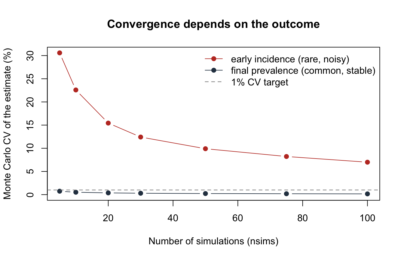
53.4 Convergence is outcome-specific
The two curves tell the whole story. Final prevalence, a count near 480, has a CV under 1% even at five replicates and reaches about 0.16% by a hundred. Early incidence, a count near three, sits at roughly 31% at five replicates and is still about 7% at a hundred, an order of magnitude short of the 1% target. Same model, same runs, wildly different precision.
The reason is the coefficient of variation itself: a rare outcome has a small mean, so the same absolute Monte Carlo noise is a large fraction of it. Rare events (uncommon deaths, subgroup-specific outcomes, tail quantities) are always the binding constraint on nsims, and they can require far more replicates than the headline outcomes, sometimes more than is feasible.
53.5 In practice
- Set
nsimsfrom the rarest outcome you need to report at your target precision, not the most common one. Sizing to prevalence alone will leave the rare contrasts underpowered. - If a rare outcome will not converge at any feasible count, report it as a directional result (which way it goes, resolved against the null) rather than as a precise magnitude, and say so.
- Remember the square-root wall: driving the CV down by another factor of two costs four times the compute. Past a point, more replicates buy very little.
- Run the convergence analysis once, on a pilot, before committing a large scenario grid to a cluster; it is cheap insurance against either noisy results or wasted node-hours.
In an HIV model with a healthcare-stigma mechanism, the common cascade and prevalence outcomes reached a 1% CV near 250 replicates, while stigma-specific subgroup outcomes converged more slowly. In a COVID-19, influenza, and RSV vaccination study on the GlobalMix networks, the infection burdens and the main transmission contrasts resolved to a 1% CV near 250 replicates, but the rare mortality contrasts were far slower: an averted-infant-death magnitude had a CV of 56% at 20 replicates and was still 11% at 500. Both studies set their production count from the rare outcomes, not the common ones.