49 Multi-Layer Networks
Real contact processes rarely happen on a single network. People have main partners and casual partners; a pathogen might spread over sexual contacts and needle-sharing contacts; students share dorm rooms and classrooms. A multi-layer network captures this: one shared set of people (the nodes), with two or more separate edge sets (the layers), each with its own formation and dissolution model. An epidemic can spread over the edges in either layer.
We build a two-layer SI epidemic in two steps, easiest first:
- Part 1: independent layers. The two layers are fit and simulated separately and simply handed to
netsim()together. If you have built a single-layer network model before, you already know almost everything here. - Part 2: dependent layers. We add the one realistic complication that makes multi-layer models genuinely different: a person’s activity in one layer constrains the other. This is where all of the new machinery lives.
Note
Download the R script to follow along here. Part 2 sources a small helper file, mod11-helpers.R, which holds the cross-layer plumbing.
NoteThe one new idea: same people, two edge sets
A layer is just a network model of the kind you have already been fitting. A multi-layer network is nothing more than two of them defined over the same nodes. Everything you know about netest, netdx, and netsim carries over, layer by layer. The only genuinely new mechanic is that you hand netsim() a list of fitted models instead of one, and it runs an epidemic that can transmit on either layer’s edges.
Part 1 does exactly that, and nothing more. Part 2 adds the single feature that couples the layers, and everything hard about multi-layer modeling lives in that one feature.
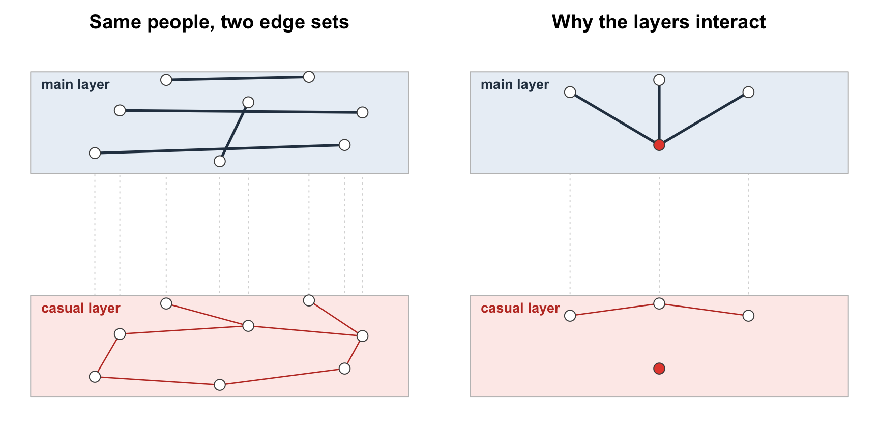
The picture below is the whole idea. On the left, one set of people carries two separate edge sets, a sparse long-lasting main layer and a denser short-lived casual layer, with the dotted lines marking the same person in each. On the right is the one complication Part 2 adds: the layers can interact, because a person busy in one layer tends to be sparse in the other.
49.1 Setup
One shared node set carries both layers. We attach a binary race attribute for homophily in the main layer.
49.2 Part 1: Independent Layers
Nothing here is new. A layer is just a network model; the only new idea is keeping two of them for the same people.
We fit two ordinary single-layer TERGMs:
- Layer 1 (main): steady, long-lasting ties (mean duration 200) with race homophily.
- Layer 2 (casual): short, high-turnover ties (mean duration 20), driven by a degree-1 target.
Layer 2’s formation references only its own structure (degree(1)), not layer 1. That independence is exactly what lets us skip all of the cross-layer machinery until Part 2.
Each layer is diagnosed on its own, exactly as any single-layer model.
Code
Now the epidemic. The one multi-layer step is netsim(list(est1, est2), ...): passing a list of fitted models. The list order sets the layer numbering (est1 is layer 1). resimulate.network = TRUE redraws both dynamic layers each step, and the optional multilayer() wrapper lets us monitor a separate set of network statistics for each layer.
Code
param   <- param.net(inf.prob = 0.5, act.rate = 2)
init    <- init.net(i.num = 10)
control <- control.net(type = "SI", nsteps = nsteps, nsims = nsims, ncores = ncores,
                       tergmLite = TRUE, resimulate.network = TRUE,
                       nwstats.formula = multilayer(~edges + nodematch("race"),
                                                    ~edges + degree(0:3)),
                       verbose = FALSE)

sim.ind <- netsim(list(est1, est2), param, init, control)
And we plot the epidemic, which is the whole point, and which single-layer intuition already prepares you to read. We do not set mean.col: with more than one outcome, plot.netsim gives each its own coordinated mean-and-band color.
Code
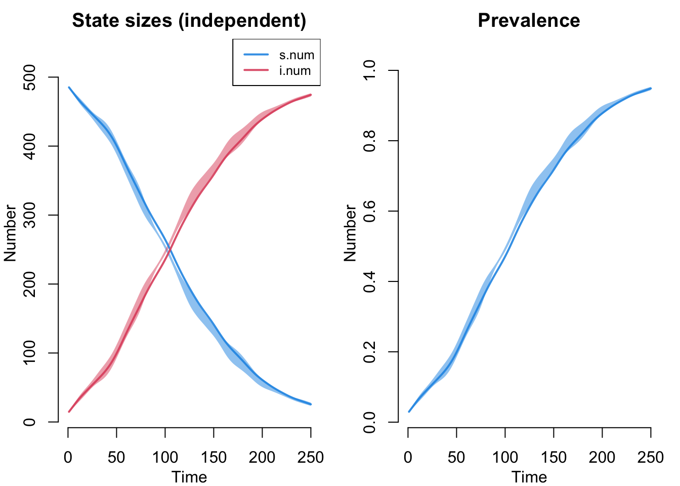
The short-duration casual layer drives early spread, while the long-duration main layer sustains transmission over time. Because either layer can transmit, the epidemic reflects both.
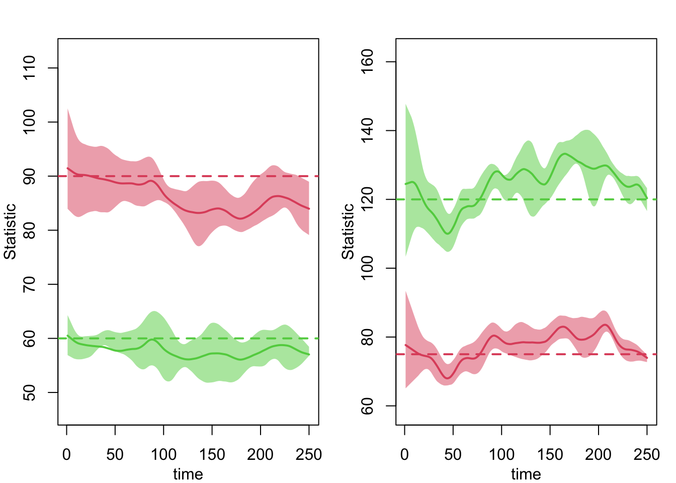
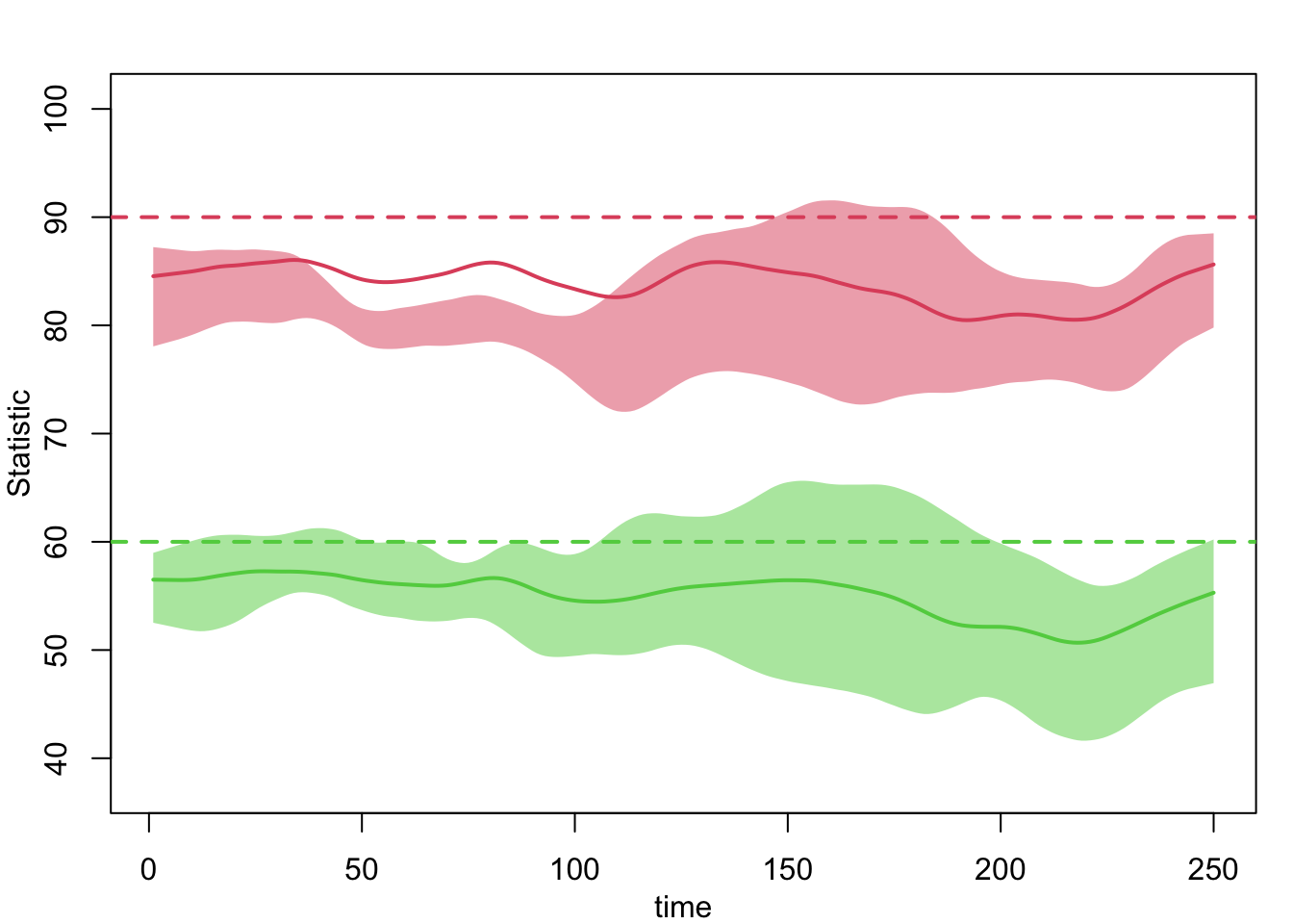
Because we passed a multilayer() nwstats.formula, netsim also monitored each layer’s formation statistics over the run. Plotting them is the network-side payoff: it confirms that both dynamic layers held their target structure while the epidemic ran on top of them.
49.3 Part 2: Dependent Layers
Part 1’s layers ignore each other, which allows something unrealistic: a person can be a hub in both the main and the casual layer at once. In reality people have finite relational capacity, so being busy in one partnership type tends to reduce activity in the other. That produces a negative cross-layer degree correlation, and reproducing it is the single decision that separates a dependent multi-layer model from an independent one.
NoteCoupling the layers creates two problems to solve
We couple the layers by adding, to each layer’s formation model, a term that reads the other layer’s degree: nodefactor("deg1+.net2") in layer 1 and nodefactor("deg1+.net1") in layer 2, each with a small target so that few nodes are active in both. That one-line addition creates two chicken-and-egg problems, and naming them separately is the key to not getting lost:
- A cold start. Layer 1’s model wants each node’s layer-2 degree, but layer 2 does not exist yet, and vice versa. We have to seed plausible starting degrees before fitting anything.
- Staying current. During the simulation each layer’s degree changes every step, so the other layer’s model must be shown the updated value each time, or the coupling silently freezes at its starting values.
We solve the first with a san() bootstrap, which is one-time setup and lives in mod11-helpers.R, and the second with a short per-step callback that we write out below.
49.3.1 The cold-start bootstrap
init_cross_degree() runs the san() (simulated annealing) seeding described above and returns the network with the two cross-layer attributes attached. Open the helper file to see exactly what it does; here we just call it.
49.3.2 Estimate the dependent layers
The formation models are Part 1’s plus one cross-layer nodefactor term each, and the targets gain one small statistic (10 of the 90 or 75 edges) that forces the negative correlation. The durations are unchanged, so the only difference from Part 1 is the coupling.
Code
est.1 <- netest(nw, ~edges + nodematch("race") + nodefactor("deg1+.net2"),
                target.stats = c(90, 60, 10),
                coef.diss = dissolution_coefs(~offset(edges), duration = 200))

est.2 <- netest(nw, ~edges + degree(1) + nodefactor("deg1+.net1"),
                target.stats = c(75, 120, 10),
                coef.diss = dissolution_coefs(~offset(edges), duration = 20))
Read the fitted models with summary(), the same tool you have used on network models since earlier in the course. The cross-layer nodefactor row is the one that matters here:
Call:
ergm(formula = formation, constraints = constraints, offset.coef = coef.form,
    target.stats = target.stats, eval.loglik = FALSE, control = set.control.ergm,
    verbose = verbose, basis = nw)

Maximum Likelihood Results:

                        Estimate Std. Error MCMC % z value Pr(>|z|)
edges                    -7.1299     0.1862      0 -38.288  < 1e-04 ***
nodematch.race            0.6964     0.2237      0   3.113  0.00185 **
nodefactor.deg1+.net2.1  -1.8305     0.3255      0  -5.624  < 1e-04 ***
---
Signif. codes:  0 '***' 0.001 '**' 0.01 '*' 0.05 '.' 0.1 ' ' 1
Log-likelihood was not estimated for this fit. To get deviances, AIC, and/or BIC, use ‘*fit* <-logLik(*fit*, add=TRUE)’ to add it to the object or rerun this function with eval.loglik=TRUE.
Dissolution Coefficients
=======================
Dissolution Model: ~offset(edges)
Target Statistics: 200
Crude Coefficient: 5.293305
Mortality/Exit Rate: 0
Adjusted Coefficient: 5.293305Call:
ergm(formula = formation, constraints = constraints, offset.coef = coef.form,
target.stats = target.stats, eval.loglik = FALSE, control = set.control.ergm,
verbose = verbose, basis = nw)
Monte Carlo Maximum Likelihood Results:
Estimate Std. Error MCMC % z value Pr(>|z|)
edges -7.2285 0.2307 0 -31.331 <1e-04 ***
degree1 0.3482 0.1623 0 2.146 0.0319 *
nodefactor.deg1+.net1.1 -1.8202 0.3569 0 -5.100 <1e-04 ***
---
Signif. codes: 0 '***' 0.001 '**' 0.01 '*' 0.05 '.' 0.1 ' ' 1Log-likelihood was not estimated for this fit. To get deviances, AIC, and/or BIC, use ‘*fit* <-logLik(*fit*, add=TRUE)’ to add it to the object or rerun this function with eval.loglik=TRUE.
Dissolution Coefficients
=======================
Dissolution Model: ~offset(edges)
Target Statistics: 20
Crude Coefficient: 2.944439
Mortality/Exit Rate: 0
Adjusted Coefficient: 2.944439
The cross-layer coefficient (nodefactor.deg1+.net2 in layer 1, nodefactor.deg1+.net1 in layer 2) is negative in both: a partner in the other layer suppresses partnering here. That negative sign is the whole point of Part 2.
49.3.3 Keep the cross-layer degree current during the simulation
Each step, netsim resimulates the two layers in turn, and each layer’s formation model reads the other layer’s current degree. If that degree is not refreshed between the resimulations it freezes at its starting value and the coupling silently switches off. The fix is a short callback that netsim calls at set points each step (flagged by the network argument), pulling each layer’s current edgelist with get_edgelist() and recomputing the “has a partner in the other layer” attribute:
Code
network_layer_updates <- function(dat, at, network) {
  if (network == 0) {          # before layer 1 is redrawn: refresh from layer 2's edges
    dat <- set_attr(dat, "deg1+.net2", pmin(get_degree(get_edgelist(dat, network = 2)), 1))
  } else if (network == 1) {   # before layer 2 is redrawn: refresh from layer 1's edges
    dat <- set_attr(dat, "deg1+.net1", pmin(get_degree(get_edgelist(dat, network = 1)), 1))
  } else if (network == 2) {   # after layer 2 is redrawn: refresh for the summary stats
    dat <- set_attr(dat, "deg1+.net2", pmin(get_degree(get_edgelist(dat, network = 2)), 1))
  }
  dat
}
49.3.4 Simulate with the cross-layer callback
The control settings are Part 1’s plus dat.updates = network_layer_updates, which wires the callback into the run.
Code
control <- control.net(type = "SI", nsteps = nsteps, nsims = nsims, ncores = ncores,
                       tergmLite = TRUE, resimulate.network = TRUE,
                       dat.updates = network_layer_updates,
                       nwstats.formula = multilayer("formation",
                         ~edges + nodefactor("deg1+.net1") + degree(0:4)),
                       verbose = FALSE)

sim.dep <- netsim(list(est.1, est.2), param, init, control)
sim.dep <- mutate_epi(sim.dep, prev = i.num / num)
49.4 The Payoff: Does the Coupling Matter?
We built the dependency to be more realistic, but does it change the epidemic? Overlay the two prevalence curves.
Code
par(mfrow = c(1, 1), mar = c(3, 3, 2, 1), mgp = c(2, 1, 0))
plot(sim.ind, y = "prev", mean.col = "steelblue", mean.lwd = 3, qnts = FALSE,
     ylim = c(0, 1), main = "Prevalence: independent vs dependent layers",
     ylab = "Prevalence", xlab = "Time step")
plot(sim.dep, y = "prev", mean.col = "firebrick", mean.lwd = 3, qnts = FALSE,
     add = TRUE)
legend("bottomright", c("Independent layers", "Dependent layers"), lwd = 3,
       col = c("steelblue", "firebrick"), bty = "n")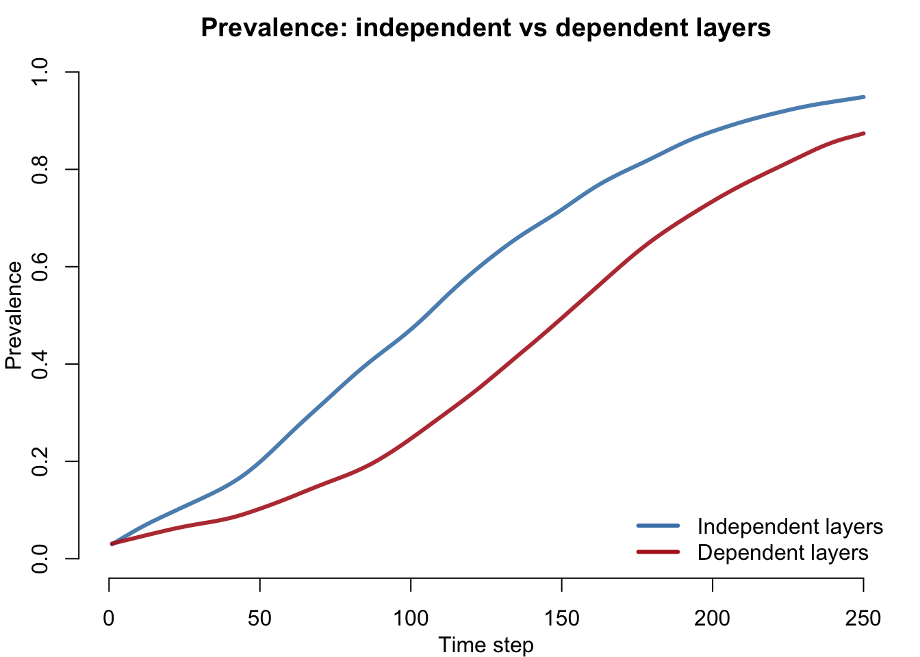
Under dependence the high-activity nodes in the two layers no longer coincide, so there are fewer people who bridge both partnership types and carry the pathogen between them. The plumbing of Part 2 is therefore not decoration: it changes which nodes do the transmitting, and so it changes the epidemic. Tying the network mechanics back to an epidemiological difference like this is the reason to bother with the dependent model at all.
49.5 Extension: Which Layer Drives Transmission?
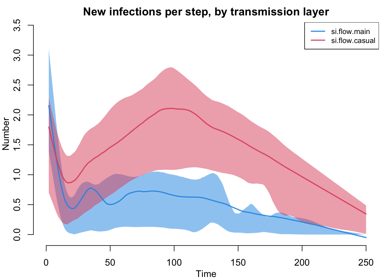
A natural research question for a multi-layer model is what share of infections happens over each layer: are most new cases coming from the long main partnerships or the churning casual ones? The built-in SI module does not record this, because it transmits over both layers at once and reports a single si.flow. To split the count we replace the transmission module with a small custom one that walks the layers separately and attributes each new infection to the layer whose edge reached it.
This is the extension API from Module 9 applied to the infection step: read the state, do the process (here, once per layer), write it back, and record two new summary statistics with set_epi().
Code
infect_bylayer <- function(dat, at) {
  status    <- get_attr(dat, "status")
  infTime   <- get_attr(dat, "infTime")
  inf.prob  <- get_param(dat, "inf.prob")
  act.rate  <- get_param(dat, "act.rate")
  finalProb <- 1 - (1 - inf.prob)^act.rate

  already <- integer(0)                 # infected this step, credited to the first layer that reached them
  count   <- c(main = 0, casual = 0)

  for (k in 1:2) {
    del <- discord_edgelist(dat, at, network = k)      # susceptible-infected pairs on layer k
    if (is.null(del)) next
    del <- del[!(del$sus %in% already), , drop = FALSE]
    if (nrow(del) == 0) next
    newly <- setdiff(unique(del$sus[rbinom(nrow(del), 1, finalProb) == 1]), already)
    if (length(newly) > 0) {
      status[newly]  <- "i"
      infTime[newly] <- at
      already  <- c(already, newly)
      count[k] <- length(newly)
    }
  }

  dat <- set_attr(dat, "status", status)
  dat <- set_attr(dat, "infTime", infTime)
  dat <- set_epi(dat, "si.flow.main",   at, count[1])
  dat <- set_epi(dat, "si.flow.casual", at, count[2])
  dat
}
We run the independent model again, but pass type = NULL and our module in the infection.FUN slot so netsim uses ours instead of the built-in transmission:
Now the by-layer flows are in the output. Plot them and read off the overall share:
Code
Code
  main casual
  0.26   0.74
The printed shares tell you where transmission concentrated. Which layer dominates depends on the interplay of mean degree and duration: a denser, faster-churning layer reaches more distinct susceptibles, while a long-lasting layer keeps re-exposing the same partners. The point is the recipe, not the specific split: once each infection is attributed to a layer, “what fraction of transmission happens where” is a one-line set_epi() away.
49.6 When Do I Need Which?
The whole module reduces to one decision and a short checklist.
| Independent layers | Dependent layers | |
|---|---|---|
| Use when | activity in one layer does not constrain the other | finite relational capacity couples the layers |
| Formation | each layer references only its own structure | add a nodefactor("deg1+.netX") cross-term per layer |
| Before fitting | nothing extra | san() bootstrap to seed the cross-layer degree (init_cross_degree()) |
| During simulation | nothing extra | per-step callback to refresh it (dat.updates = network_layer_updates) |
| The multi-layer step | netsim(list(est1, est2), ...) |
the same: netsim(list(est.1, est.2), ...) |
One-line rule: independent = a list of netest calls; dependent = add a cross-layer term, a san() seed, and a dat.updates callback.
49.7 Key EpiModel Functions for Multi-Layer Models
| Function / argument | Purpose |
|---|---|
netsim(list(est1, est2), ...) |
a list of fitted models is what makes a model multi-layer; list order sets the layer number |
resimulate.network = TRUE |
redraw both dynamic layers each step |
tergmLite = TRUE |
lightweight edgelist representation; required for the current-edgelist access (get_edgelist(dat, network = k)) the callback uses |
nwstats.formula = multilayer(f1, f2) |
monitor a separate set of network statistics for each layer |
dat.updates = <fn> |
per-step callback (dependent layers only) that refreshes the cross-layer attributes |
49.8 Your Turn
Put these models to work in the Multi-Layer Networks Lab. You will re-time a layer to show that duration, not just formation, drives the epidemic; predict and then check whether the cross-layer coupling changes peak prevalence; use the by-layer tracker above to ask where transmission happens under independence versus dependence; and add a third layer for the price of one more netest. A worked solution accompanies the lab.