51  Appendix: Epidemics over Observed Networks

Everything in the course so far has followed one workflow: observe a network egocentrically (a sample of nodes and their partnerships), fit a temporal ERGM with netest, and simulate an epidemic from that fitted model. The fit is what lets a small sample stand in for a whole population, and what lets the network keep evolving during the run.

Sometimes you do not need the fit. If you have a dynamic network census, every node and every partnership directly observed over a series of time steps, you already have the object netsim would otherwise have to generate. This chapter shows the alternative workflow: place the observed networkDynamic object straight into the simulation and run the epidemic over it, with no ERGM estimation at all.

NoteThe one idea: skip the fit when the network is fully observed

netest exists to turn partial, egocentric data into a generative model you can simulate from. A full dynamic census is not partial, so there is nothing to estimate. You hand netsim the observed network, tell it not to regenerate the network each step (resimulate.network = FALSE), and supply two small custom modules so EpiModel reads from the observed object instead of from a model fit. Everything else, the transmission process, the trackers, the plots, is the EpiModel you already know.

This is the one workflow in the course that bypasses the ERGM pipeline entirely. It is the right tool when the network really is observed in full over time (some contact-tracing, sensor, or animal-tracking datasets are), and the wrong tool when you have a sample and want to generalize from it, which is the far more common case and the reason the rest of the course teaches estimation.

For the opposite end of the same pipeline, see Module 10, where a small egocentric sample has to be reconciled into target statistics before anything can be fit. Reading the two together shows what estimation is actually buying: everything Module 10 spends its effort on, balance and degrees of freedom, is work a full census makes unnecessary.

Note

Download the R script to follow along here.

51.1 Setup

We use a simulated dynamic network from the networkDynamicData package and treat it as if it were an observed census. The network is 1000 nodes with edge spells (onset and terminus times for each partnership) recorded over roughly 100 discrete time steps.

library(EpiModel)
library(networkDynamicData)
set.seed(12345)

nsims  <- 5
ncores <- 5
nsteps <- 100

51.2 Two Custom Modules

Because there is no model fit, EpiModel’s built-in initialization and infection modules, which both expect a netest object, do not apply. We replace them with two functions that work from the observed network directly. Both follow the read-process-write module contract from Module 9.

51.2.1 Initialization

init_obsnw replaces the built-in initialize.net. It builds the master data object, drops the observed networkDynamic straight into it, seeds the initial infections, and (optionally) stores disease status on the network as a temporally extended attribute so we can color network plots by status later.

init_obsnw <- function(x, param, init, control, s) {

  dat <- create_dat_object(param, init, control)

  dat$num.nw <- 1L
  dat$run$nw[[1]] <- x                              # the observed network goes in as-is
  dat <- set_param(dat, "groups", 1)

  i.num <- get_init(dat, "i.num")
  n <- network.size(dat$run$nw[[1]])
  dat <- append_core_attr(dat, 1, n)

  status <- rep("s", n)
  status[sample(1:n, i.num)] <- "i"                 # seed i.num random infections
  dat <- set_attr(dat, "status", status)

  infTime <- rep(NA, n)
  infTime[which(status == "i")] <- 1
  dat <- set_attr(dat, "infTime", infTime)

  track.nw.attr <- get_param(dat, "track.nw.attr", override.null.error = TRUE)
  if (!is.null(track.nw.attr) && track.nw.attr) {
    dat$run$nw[[1]] <- networkDynamic::activate.vertex.attribute(
      dat$run$nw[[1]], prefix = "testatus",
      value = get_attr(dat, "status"), onset = 1, terminus = Inf
    )
  }

  dat <- prevalence.net(dat, 1)
  return(dat)
}

51.2.2 Infection

infect_obsnw handles transmission. It reads the discordant (susceptible-infectious) partnerships active at the current step off the observed network with discord_edgelist(), exactly as a normal infection module would, and draws transmission. It supports two modes: a constant per-act probability (inf.prob), or a two-stage, duration-dependent probability (inf.prob.stage1 / inf.prob.stage2), selected automatically by which parameters you supplied.

infect_obsnw <- function(dat, at) {

  active  <- get_attr(dat, "active")
  status  <- get_attr(dat, "status")
  infTime <- get_attr(dat, "infTime")

  act.rate <- get_param(dat, "act.rate")
  inf.prob.stage1 <- get_param(dat, "inf.prob.stage1", override.null.error = TRUE)

  time_varying <- !is.null(inf.prob.stage1)
  if (time_varying) {
    inf.prob.stage2 <- get_param(dat, "inf.prob.stage2")
    dur.stage1 <- get_param(dat, "dur.stage1")
  } else {
    inf.prob <- get_param(dat, "inf.prob")
  }

  idsInf <- which(active == 1 & status == "i")
  nActive <- sum(active == 1)
  nElig <- length(idsInf)

  totInf <- 0

  if (nElig > 0 && nElig < nActive) {

    del <- discord_edgelist(dat, at)                # SI pairs active on the observed network

    if (!is.null(del)) {

      if (time_varying) {
        infDur.del <- at - infTime[del$inf]
        del$transProb <- ifelse(infDur.del <= dur.stage1,
                                inf.prob.stage1, inf.prob.stage2)
      } else {
        del$transProb <- inf.prob
      }

      del$actRate <- act.rate
      del$finalProb <- 1 - (1 - del$transProb) ^ del$actRate
      transmit <- rbinom(nrow(del), 1, del$finalProb)
      del <- del[which(transmit == 1), ]

      idsNewInf <- unique(del$sus)
      totInf <- length(idsNewInf)

      if (totInf > 0) {
        status[idsNewInf] <- "i"
        infTime[idsNewInf] <- at
        dat <- set_attr(dat, "status", status)
        dat <- set_attr(dat, "infTime", infTime)

        track.nw.attr <- get_param(dat, "track.nw.attr", override.null.error = TRUE)
        if (!is.null(track.nw.attr) && track.nw.attr) {
          dat$run$nw[[1]] <- networkDynamic::activate.vertex.attribute(
            dat$run$nw[[1]], prefix = "testatus",
            value = "i", onset = at, terminus = Inf, v = idsNewInf
          )
        }
      }
    }
  }

  dat <- set_epi(dat, "si.flow", at, totInf)
  return(dat)
}

51.3 Loading the Observed Network

The concurrencyComparisonNets dataset provides an observed dynamic network as its base object. We remove its pre-recorded disease status attribute, since we simulate our own epidemic on top of the observed contact structure.

data(concurrencyComparisonNets)
nw <- base
nw <- network::delete.vertex.attribute(nw, "status.active")
print(nw)

NetworkDynamic properties:
  distinct change times: 102 
  maximal time range: -Inf until  Inf 

Includes optional net.obs.period attribute:
 Network observation period info:
  Number of observation spells: 1 
  Maximal time range observed: 2 until 102 
  Temporal mode: discrete 
  Time unit: step 
  Suggested time increment: 1 

 Network attributes:
  vertices = 1000 
  directed = FALSE 
  hyper = FALSE 
  loops = FALSE 
  multiple = FALSE 
  bipartite = FALSE 
  net.obs.period: (not shown)
  total edges= 1916 
    missing edges= 0 
    non-missing edges= 1916 

 Vertex attribute names: 
    vertex.names 

 Edge attribute names not shown 

51.4 Example 1: A Basic SI Epidemic

The first run is a plain SI model: a constant 50% per-act transmission probability and one act per partnership per step.

param <- param.net(inf.prob = 0.5, act.rate = 1)
init  <- init.net(i.num = 10)

The control settings are where the observed-network workflow shows itself. We pass our two custom modules, keep the built-in prevalence.net recorder, and set resimulate.network = FALSE so the observed edges are used as-is. There is no ERGM fit to compute network statistics from, so we turn off save.nwstats. Critically, nsteps matches the number of observed time steps in the network.

control <- control.net(
  type = NULL,
  nsteps = nsteps,
  nsims = nsims,
  ncores = ncores,
  initialize.FUN = init_obsnw,
  infection.FUN = infect_obsnw,
  prevalence.FUN = prevalence.net,
  resimulate.network = FALSE,
  save.nwstats = FALSE,
  verbose = FALSE
)

Note that the first argument to netsim is the observed network nw, not a fitted netest object. That substitution is the whole point.

sim <- netsim(nw, param, init, control)

sim

EpiModel Simulation
=======================
Model class: netsim

Simulation Summary
-----------------------
Model type:
No. simulations: 5
No. time steps: 100
No. NW groups: 1

Fixed Parameters
---------------------------
inf.prob = 0.5
act.rate = 1
groups = 1

Model Functions
-----------------------
initialize.FUN 
resim_nets.FUN 
summary_nets.FUN 
infection.FUN 
nwupdate.FUN 
prevalence.FUN 
verbose.FUN 

Model Output
-----------------------
Variables: s.num i.num num si.flow
Networks: sim1 ... sim5
Transmissions: sim1 ... sim5

51.5 A Caveat: Match nsteps to the Observation Window

The observed network has edge activity recorded over a finite window of about 100 steps. By a networkDynamic convention, edges active at the last observed time stay active indefinitely, so nothing stops you from simulating past the window, but the results stop meaning anything: the edge set is frozen, so it no longer reflects real turnover.

You can see the frozen edges directly. The dyads active at step 100 and step 200 are identical, because nothing dissolves after the observation ends:

head(get.dyads.active(nw, at = 1),   5)

     [,1] [,2]
[1,]  834    4
[2,]  251    9
[3,]  722    9
[4,]   93   10
[5,]  169   10

head(get.dyads.active(nw, at = 100), 5)

     [,1] [,2]
[1,]  445   46
[2,]  464   78
[3,]  380  270
[4,]  777  365
[5,]  850  808

head(get.dyads.active(nw, at = 200), 5)

     [,1] [,2]
[1,]  445   46
[2,]  464   78
[3,]  380  270
[4,]  777  365
[5,]  850  808

Running 200 steps on the roughly 100-step network shows the symptom: prevalence plateaus and incidence falls to zero once the frozen structure takes over.

control_caveat <- control.net(
  type = NULL, nsteps = 200, nsims = nsims, ncores = ncores,
  initialize.FUN = init_obsnw, infection.FUN = infect_obsnw,
  prevalence.FUN = prevalence.net,
  resimulate.network = FALSE, save.nwstats = FALSE, verbose = FALSE
)
sim_caveat <- netsim(nw, param, init, control_caveat)

par(mfrow = c(1, 2), mar = c(3, 3, 2, 1), mgp = c(2, 1, 0))
plot(sim_caveat, y = "i.num", main = "Prevalence past the window",
     ylab = "Infected count", xlab = "Time step", legend = FALSE)
plot(sim_caveat, y = "si.flow", main = "Incidence past the window",
     ylab = "New infections", xlab = "Time step", legend = FALSE)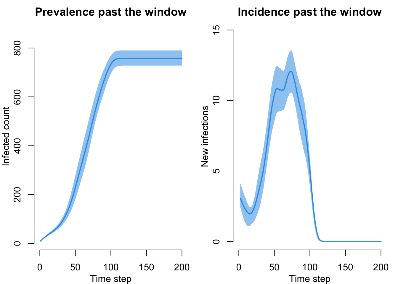

The rule is simple: match nsteps to the number of observed time steps.

51.6 Example 2: Time-Varying Transmission

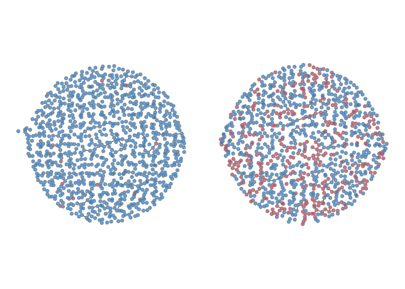
The second run uses the duration-dependent mode of the infection module. Transmission is low in the primary stage (5% per act for the first 5 steps after infection) and higher afterward (15% per act), a common shape for infections with an early low-shedding period. Setting track.nw.attr = TRUE stores disease status on the network so we can visualize it.

param <- param.net(
  inf.prob.stage1 = 0.05,
  inf.prob.stage2 = 0.15,
  dur.stage1 = 5,
  act.rate = 1,
  track.nw.attr = TRUE
)
init <- init.net(i.num = 10)

control <- control.net(
  type = NULL, nsteps = nsteps, nsims = nsims, ncores = ncores,
  initialize.FUN = init_obsnw, infection.FUN = infect_obsnw,
  prevalence.FUN = prevalence.net,
  resimulate.network = FALSE, save.nwstats = FALSE, verbose = FALSE
)

sim2 <- netsim(nw, param, init, control)

Because we tracked status on the network, we can plot the observed network colored by disease status at an early and a late step.

par(mfrow = c(1, 2), mar = c(1, 1, 1, 1))
plot(sim2, type = "network", col.status = TRUE, at = 2,      sims = 1)
plot(sim2, type = "network", col.status = TRUE, at = nsteps, sims = 1)

The same stored attribute can be read back at the individual level with the networkDynamic API, which is how you would extract who was infected when for a downstream analysis:

nwd <- get_network(sim2, 1)
head(get.vertex.attribute.active(nwd, "testatus", at = nsteps), 10)

 [1] "s" "i" "s" "i" "s" "s" "i" "s" "s" "i"

51.7 Comparing the Two Runs

The constant, high transmission of Example 1 saturates quickly; the lower, staged transmission of Example 2 climbs more slowly.

sim  <- mutate_epi(sim,  prev = i.num / num)
sim2 <- mutate_epi(sim2, prev = i.num / num)
par(mfrow = c(1, 2), mar = c(3, 3, 2, 1), mgp = c(2, 1, 0))
plot(sim,  y = "i.num", main = "Ex 1: constant transmission",
     ylab = "Infected count", xlab = "Time step", legend = FALSE)
plot(sim2, y = "i.num", main = "Ex 2: time-varying transmission",
     ylab = "Infected count", xlab = "Time step", legend = FALSE)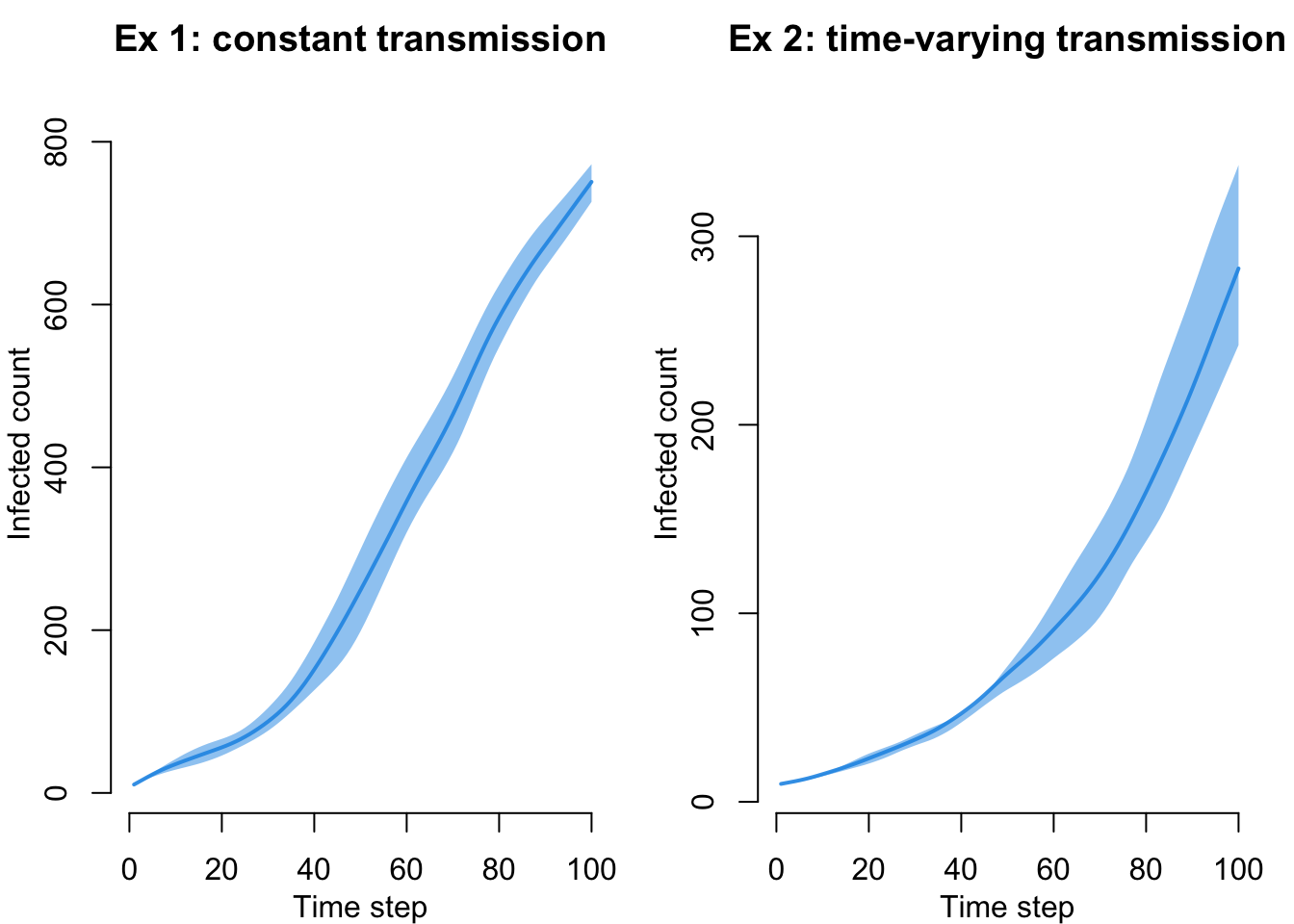

51.8 When to Use This

	Fit and simulate (the rest of the course)	Observed network (this chapter)
You have	an egocentric sample of the network	a full dynamic census of nodes and edges over time
Network step	netest fits a TERGM you simulate from	the observed networkDynamic object is used directly
resimulate.network	TRUE (the model regenerates the network)	FALSE (the observed edges are fixed)
Custom modules	usually not needed for the network itself	a custom initialize.FUN and infection.FUN
Run length	any nsteps the model supports	nsteps capped at the observation window

The estimation workflow is the general-purpose one, because full network censuses are rare and samples are the norm. Reach for the observed-network approach only when you genuinely have the whole network over time and want to run transmission on exactly that structure without a modeling layer in between.

51.9 Your Turn

• Convert the model to SIS or SIR by adding a recovery module (the Module 9 pattern), and see how the fixed observation window interacts with recovery.
• Swap in a different observed dynamic network from networkDynamicData and confirm you reset nsteps to its own observation length.
• Bridge the two workflows: take a static observed network, assume an edge dissolution rate, and fit a TERGM with netest, the approach from the Module 6 network-census lab, then contrast it with using a dynamic census directly here.