58 Starting a COVID Model

In this tutorial, we will build on our SEIR model for COVID-19 by adding demography (aging, births, and deaths). This will involve learning a few new components of the EpiModel extension API.

Note

This tutorial has two R scripts you should download: a primary script containing the code below and a separate module script. Download both and put them in the same working directory.

58.1 Setup

First start by loading EpiModel and clearing your global environment.

Code

library(EpiModel)
rm(list = ls())

We will use the extension infection and disease progression modules from Day 4. Like the models with extension modules we ran then, we will keep the functions within one R script and the code to run the model in another script. For the purposes of this tutorial, we will show them bundled together but the linked files are split.

We will start with the initialization of the network object, with the relevant age and disease status attributes, then show the new epidemic models, then the network model estimation, and then epidemic model parameterization and simulation. In practice, we would typically go back and forth many times between all of these components.

58.2 Network Initialization

The model will represent age as a continuous nodal attribute. Aging will increment this attribute for everyone by a day (the value of the time step) in a linear fashion, and mortality will be a function of age.

To start, we initialize the range of possible ages (in years) at the outset.

Code

ages <- 0:85

Next, we calculate age-specific mortality rates based on one demographic table online. This lists the rates per year per 100,000 persons in the United States by age groups, in the following age bands:

Code

# Rates per 100,000 for age groups: <1, 1-4, 5-9, 10-14, 15-19, 20-24, 25-29,
#                                   30-34, 35-39, 40-44, 45-49, 50-54, 55-59,
#                                   60-64, 65-69, 70-74, 75-79, 80-84, 85+
departure_rate <- c(588.45, 24.8, 11.7, 14.55, 47.85, 88.2, 105.65, 127.2,
                    154.3, 206.5, 309.3, 495.1, 736.85, 1051.15, 1483.45,
                    2294.15, 3642.95, 6139.4, 13938.3)

To convert this to a per-capita daily death rate, we divide by 365,000:

Code

dr_pp_pd <- departure_rate / 1e5 / 365

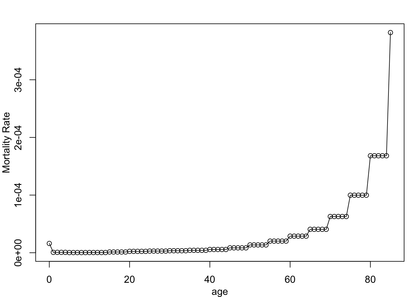
Next we build out a vector of daily death rates by repeating the rate above by the size of the age band. Now we have a rate for each age, with some repeats within age band.

Code

age_spans <- c(1, 4, rep(5, 16), 1)
dr_vec <- rep(dr_pp_pd, times = age_spans)
head(data.frame(ages, dr_vec), 20)

   ages       dr_vec
1     0 1.612192e-05
2     1 6.794521e-07
3     2 6.794521e-07
4     3 6.794521e-07
5     4 6.794521e-07
6     5 3.205479e-07
7     6 3.205479e-07
8     7 3.205479e-07
9     8 3.205479e-07
10    9 3.205479e-07
11   10 3.986301e-07
12   11 3.986301e-07
13   12 3.986301e-07
14   13 3.986301e-07
15   14 3.986301e-07
16   15 1.310959e-06
17   16 1.310959e-06
18   17 1.310959e-06
19   18 1.310959e-06
20   19 1.310959e-06

It ends up looking like this visually:

Code

par(mar = c(3,3,2,1), mgp = c(2,1,0), mfrow = c(1,1))
plot(ages, dr_vec, type = "o", xlab = "age", ylab = "Mortality Rate")

We will now add age and disease status attributes to an initialized network object. We will use a larger population size than last time:

Code

n <- 1000
nw <- network_initialize(n)

For each node, we will randomly sample an age from the vector of ages (from 0 to 85), and then set that as a vertex attribute on the network object.

Code

ageVec <- sample(ages, n, replace = TRUE)
nw <- set_vertex_attribute(nw, "age", ageVec)

This model will also initialize people into a latent (E state) disease stage.

Code

statusVec <- rep("s", n)
init.latent <- sample(1:n, 50)
statusVec[init.latent] <- "e"
table(statusVec)

statusVec
  e   s 
 50 950

Code

which(statusVec == "e")

 [1]  23  39  59  65  76 117 139 147 182 192 205 240 256 264 267 282 307 313 326
[20] 331 369 370 371 405 408 454 469 542 619 632 642 694 698 717 741 752 769 798
[39] 799 804 810 838 841 857 867 905 919 920 929 962

Because of that we will manually set up a vector of disease statuses and set it on the network object as a status attribute. This is an alternative way to set up disease status, instead of using the initial conditions in init.net.

Code

nw <- set_vertex_attribute(nw, "status", statusVec)
nw

 Network attributes:
  vertices = 1000 
  directed = FALSE 
  hyper = FALSE 
  loops = FALSE 
  multiple = FALSE 
  bipartite = FALSE 
  total edges= 0 
    missing edges= 0 
    non-missing edges= 0 

 Vertex attribute names: 
    age status vertex.names 

No edge attributes

58.3 Demographic Modules

With the network initialized, we will now turn to building out the three new extension modules. This set of extensions will add three demographic processes to the model: aging, births, and deaths. The birth and death processes in particular will involve some specific changes to the nodes that must be completed under the EpiModel extension API.

The same three processes (aging on a life table, births, and age-specific deaths) are maintained as a standalone Gallery example, SI with Age-Specific Vital Dynamics. We keep the code inline here because we step through it live in class, but that Gallery example is the maintained, CI-tested copy to reuse and adapt in practice.

58.3.1 Aging

The aging module performs one simple process: to update the age attribute (in years) of everyone on the network by a day (or 1/365 years). It does this by getting the age attribute from the dat object, updating the vector, and then setting it back on the dat object. The function design follows the same format as our SEIR modules in Day 4.

Code

aging <- function(dat, at) {

  age <- get_attr(dat, "age")
  age <- age + 1/365
  dat <- set_attr(dat, "age", age)

  dat <- set_epi(dat, "meanAge", at, mean(age, na.rm = TRUE))

  return(dat)
}

We also add a new summary statistic, meanAge, which is the mean of the age vector for that time step.

58.3.2 Mortality

For the mortality module, we will implement a process of age-specific mortality with an excess risk of death with active infection. The process is more complex than the built-in departures module (which might cover death but other forms of exit from the population). We will step through the function together in the tutorial.

Note that the overall design of the function is similar to any other EpiModel extension module. The get_ and set_ functions are used to read and write to the dat object. The individual process of mortality involves querying the death rates by the age of active nodes, and then drawing from a binomial distribution for each eligible node.

EpiModel API Rule: A departure module must set the active attribute to 0 and the exitTime attribute to the current step at for every departing node, which is how EpiModel knows to update the network at the end of the step. The full attribute-bookkeeping contract is documented in the Working with Custom Attributes and Summary Statistics vignette and follows the extension API introduced in Module 9.

Code

dfunc <- function(dat, at) {

  ## Attributes
  active <- get_attr(dat, "active")
  exitTime <- get_attr(dat, "exitTime")
  age <- get_attr(dat, "age")
  status <- get_attr(dat, "status")

  ## Parameters
  dep.rates <- get_param(dat, "departure.rates")
  dep.dis.mult <- get_param(dat, "departure.disease.mult")

  ## Query alive
  idsElig <- which(active == 1)
  nElig <- length(idsElig)

  ## Initialize trackers
  nDepts <- 0
  idsDepts <- NULL

  if (nElig > 0) {

    ## Calculate age-specific departure rates for each eligible node ##
    ## Everyone older than 85 gets the final mortality rate
    whole_ages_of_elig <- pmin(ceiling(age[idsElig]), 86)
    drates_of_elig <- dep.rates[whole_ages_of_elig]

    ## Multiply departure rates for diseased persons
    idsElig.inf <- which(status[idsElig] == "i")
    drates_of_elig[idsElig.inf] <- drates_of_elig[idsElig.inf] * 
                                   dep.dis.mult

    ## Simulate departure process
    vecDepts <- which(rbinom(nElig, 1, drates_of_elig) == 1)
    idsDepts <- idsElig[vecDepts]
    nDepts <- length(idsDepts)

    ## Update nodal attributes
    if (nDepts > 0) {
      active[idsDepts] <- 0
      exitTime[idsDepts] <- at
    }
  }

  ## Set updated attributes
  dat <- set_attr(dat, "active", active)
  dat <- set_attr(dat, "exitTime", exitTime)
  
  ## Summary statistics ##
  dat <- set_epi(dat, "total.deaths", at, nDepts)

  # covid deaths
  covid.deaths <- length(intersect(idsDepts, which(status == "i")))
  dat <- set_epi(dat, "covid.deaths", at, covid.deaths)

  return(dat)
}

Note that the overall process of mortality involves flipping a coin for each eligible person in the population, weighted by their age and disease status, and keeping track of who came up as heads (i.e., a 1). We end the function by saving two summary statistics that count the overall deaths and the COVID-related deaths separately.

58.3.3 Births

Finally, we add a new arrivals module to handle births (there may be other forms of arrivals such as in-migration that we would like to handle separately) but not in this model. In terms of the process, births is a simple function of the current population size times a fixed birth rate. This is stochastic at each time step by drawing an non-negative integer from a Poisson distribution.

EpiModel API Rule: Every incoming node needs all of its nodal attributes set. append_core_attr handles the three that are uniform across models (active, entrTime, and exitTime); we set the rest with append_attr, here status, infTime, and the model-specific age, passing either a single value recycled across all arrivals or a vector with one value per arrival. The required attributes are described in the Working with Custom Attributes and Summary Statistics vignette; the append_* helpers are shown in the si-vital-dynamics Gallery example and in ?append_core_attr, extending the accessor pattern from Module 9.

Code

afunc <- function(dat, at) {

  ## Parameters ##
  n <- get_epi(dat, "num", at - 1)
  a.rate <- get_param(dat, "arrival.rate")

  ## Process ##
  nArrivalsExp <- n * a.rate
  nArrivals <- rpois(1, nArrivalsExp)

  # Update attributes
  if (nArrivals > 0) {
    dat <- append_core_attr(dat, at = at, n.new = nArrivals)
    dat <- append_attr(dat, "status", "s", nArrivals)
    dat <- append_attr(dat, "infTime", NA, nArrivals)
    dat <- append_attr(dat, "age", 0, nArrivals)
  }

  ## Summary statistics ##
  dat <- set_epi(dat, "a.flow", at, nArrivals)

  return(dat)
}

We close the function by adding a summary statistic for the number of births.

58.4 Network Model Estimation

With the new modules defined, we can return to parameterizing the network model. Recall that we have initialized the network and set the age and status attributes on the network above.

Code

nw

 Network attributes:
  vertices = 1000 
  directed = FALSE 
  hyper = FALSE 
  loops = FALSE 
  multiple = FALSE 
  bipartite = FALSE 
  total edges= 0 
    missing edges= 0 
    non-missing edges= 0 

 Vertex attribute names: 
    age status vertex.names 

No edge attributes

Next we will parameterize the model starting with the same terms as our last SEIR model, but adding an absdiff term for age. This will control the average absolute difference in ages between any two nodes. With a small target statistic, this will allow for continuous age homophily (assortative mixing).

Code

formation <- ~edges + degree(0) + absdiff("age")

For target statistics, we will start with mean degree, transform that to the expected edges, and then calculate the number of isolates (a synonym for degree(0)) as a proportion of nodes, and absdiff as a function of edges (the target statistic is the sum of all absolute differences in age across all edges, so this is the mean difference times the number of edges).

Code

mean_degree <- 2
edges <- mean_degree * (n/2)
avg.abs.age.diff <- 2
isolates <- n * 0.08
absdiff <- edges * avg.abs.age.diff

target.stats <- c(edges, isolates, absdiff)
target.stats

[1] 1000   80 2000

The dissolution model will use a standard homogeneous dissolution rate, with a death correction here based on the average death rate across the population and a multiplier to account for higher mortality due to COVID. This is not perfect, but this parameter is quite robust to misspecification because the huge differential in average relational duration versus average lifespan (1/mortality rates); notice the minimal change in coefficient with this adjustment.

Code

coef.diss <- dissolution_coefs(~offset(edges), 20, mean(dr_vec)*2)
coef.diss

Dissolution Coefficients
=======================
Dissolution Model: ~offset(edges)
Target Statistics: 20
Crude Coefficient: 2.944439
Mortality/Exit Rate: 6.31841e-05
Adjusted Coefficient: 2.946969

Next we fit the model. You can ignore any warning messages about fitted probabilities that were 0 or 1. These are standard GLM fitting messages. If there is a problem in the model fit, it will emerge in the diagnostics.

Code

est <- netest(nw, formation, target.stats, coef.diss)

We will run the model diagnostics by monitoring both the terms in the model formula and an extension of the degree terms out to degree of 6. We are using an MCMC control setting here to tweak the simulation algorithm to increase the “burn-in” for the Markov chain; this burn-in control is especially helpful in cases of ERGM formulas with absdiff terms (i.e., those with continuous attributes). Although the fit is not perfect here (we are on the cusp of where we also might want to turn off the edges dissolution approximation with edapprox), it is close enough to move forward for this tutorial.

Code

dx <- netdx(est, nsims = 10, ncores = 5, nsteps = 500,
            nwstats.formula = ~edges + absdiff("age") + degree(0:6),
            set.control.tergm = control.simulate.formula.tergm(MCMC.burnin.min = 20000))


Network Diagnostics
-----------------------
- Simulating 10 networks
- Calculating formation statistics

Code

print(dx)

EpiModel Network Diagnostics
=======================
Diagnostic Method: Dynamic
Simulations: 10
Time Steps per Sim: 500

Formation Diagnostics
----------------------- 
            Target Sim Mean Pct Diff Sim SE Z Score SD(Sim Means) SD(Statistic)
edges         1000  987.595   -1.240  1.688  -7.348         6.046        25.095
absdiff.age   2000 1995.470   -0.226  5.885  -0.770        20.588        82.227
degree0         80   90.169   12.712  0.400  25.447         1.878         9.570
degree1         NA  320.626       NA  0.729      NA         3.162        15.747
degree2         NA  290.969       NA  0.560      NA         1.638        14.437
degree3         NA  176.973       NA  0.527      NA         2.239        12.967
degree4         NA   80.182       NA  0.386      NA         1.461         9.310
degree5         NA   29.337       NA  0.197      NA         0.687         5.368
degree6         NA    8.737       NA  0.111      NA         0.427         3.010

Duration Diagnostics
----------------------- 
      Target Sim Mean Pct Diff Sim SE Z Score SD(Sim Means) SD(Statistic)
edges     20   20.033    0.166  0.053   0.621         0.232         0.668

Dissolution Diagnostics
----------------------- 
      Target Sim Mean Pct Diff Sim SE Z Score SD(Sim Means) SD(Statistic)
edges   0.05     0.05   -0.089      0  -0.499             0         0.007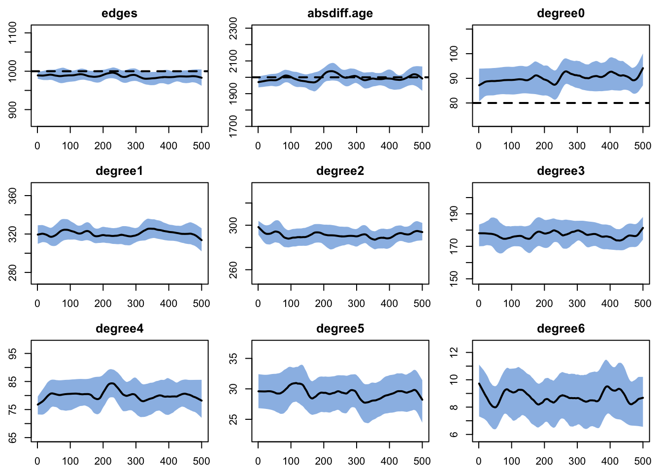

Code

plot(dx)

58.5 EpiModel Model Simulation

To parameterize the model, we need to add the newly referenced model parameters to param.net. These include the departure and arrival rates. Although our past parameters have been scalars (single values), there is nothing to prevent us from passing vectors (or even more structured objects like lists or data frames) as parameters. That is what we do with departure.rates. The departure.disease.mult is the multiplier on the base death rate for persons with active infection (persons in the “i” status). We will assume the arrival rate reflects the average lifespan in days.

Code

param <- param.net(inf.prob = 0.1,
                   act.rate = 3,
                   departure.rates = dr_vec,
                   departure.disease.mult = 100,
                   arrival.rate = 1/(365*85),
                   ei.rate = 0.05, ir.rate = 0.05)

For initial conditions, we have passed in the number initially in the latent state at the outset, so init.net just needs to be a placeholder input.

Code

init <- init.net()

Finally, for control settings, we first source in the new function script (this should now contain five extension functions), and include module names and associated functions for each of the five. Note that these five modules will run in addition to the standard modules that handle initialization, network resimulation, and so on. For this model, we definitely want to resimulate the network at each time step, and we will use tergmLite for computational efficiency. We again use a burn-in control setting for TERGM simulations here, plus add some additional network statistics to monitor for diagnostics.

Code

source("mod13-COVID1-fx.R")
control <- control.net(type = NULL,
                       nsims = 5,
                       ncores = 5,
                       nsteps = 300,
                       infection.FUN = infect,
                       progress.FUN = progress,
                       aging.FUN = aging,
                       departures.FUN = dfunc,
                       arrivals.FUN = afunc,
                       resimulate.network = TRUE,
                       tergmLite = TRUE,
                       set.control.tergm = control.simulate.formula.tergm(MCMC.burnin.min = 10000),
                       nwstats.formula = ~edges + meandeg + degree(0:2) + absdiff("age"))

With all that complete, we now are ready to run netsim. This should take a minute.

Code

sim <- netsim(est, param, init, control)

58.6 Post-Simulation Diagnostics

We run the network diagnostics with the netsim simulations complete to evaluate the potential impact of the epidemic processes on the network diagnostics. Here we see that the three targeted statistics are not maintained at their target levels. Part of this may be due to the general bias in the fit introduced by the edges dissolution approximation, highlighted in the netdx diagnostics above. But the change to the edges and absdiff statistics may be concerning.

Code

plot(sim, type = "formation",
     stats = c("edges", "absdiff.age", "degree0"), plots.joined = FALSE)

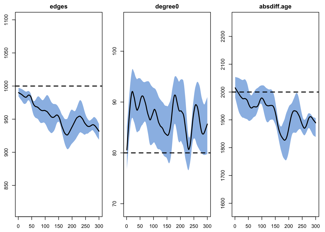
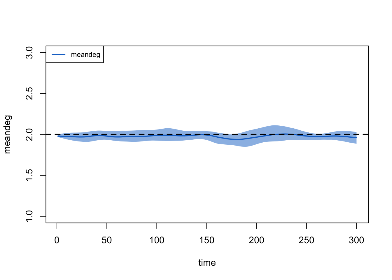
However, it is important to note that the change in edges may be related to underlying reductions in the population size (as a function of relatively high COVID-related mortality). To demonstrate this, we examine the meandeg statistics, which is the per capita mean degree (i.e., it does not depend on the fluctuations in population size). Here, the target statistic is relatively stable (perhaps a minor bias but nothing that will influence the epi outcomes too much).

Code

plot(sim, type = "formation", stats = "meandeg", qnts = 1, ylim = c(1, 3))
abline(h = 2, lty = 2, lwd = 2)

58.7 Epidemic Model Analysis

With the epidemic model simulation complete, let’s inspect the network object. We can see a listing of the modules used, and the model output variables available for inspection. Because we used tergmLite, we only have the summary statistic data and not the individual-level network data.

Code

sim

EpiModel Simulation
=======================
Model class: netsim

Simulation Summary
-----------------------
Model type:
No. simulations: 5
No. time steps: 300
No. NW groups: 1

Fixed Parameters
---------------------------
inf.prob = 0.1
act.rate = 3
departure.rates = 1.612192e-05 6.794521e-07 6.794521e-07 6.794521e-07 
6.794521e-07 3.205479e-07 3.205479e-07 3.205479e-07 3.205479e-07 3.205479e-07 
...
departure.disease.mult = 100
arrival.rate = 3.223207e-05
ei.rate = 0.05
ir.rate = 0.05
groups = 1

Model Functions
-----------------------
initialize.FUN 
resim_nets.FUN 
summary_nets.FUN 
infection.FUN 
departures.FUN 
arrivals.FUN 
nwupdate.FUN 
prevalence.FUN 
verbose.FUN 
progress.FUN 
aging.FUN 

Model Output
-----------------------
Variables: s.num i.num num ei.flow ir.flow e.num r.num 
meanAge se.flow total.deaths covid.deaths a.flow
Networks: sim1 ... sim5
Transmissions: sim1 ... sim5

Formation Statistics
----------------------- 
            Target Sim Mean Pct Diff Sim SE Z Score SD(Sim Means) SD(Statistic)
edges         1000  955.253   -4.475  4.604  -9.719        16.573        33.280
meandeg         NA    1.977       NA  0.006      NA         0.024         0.054
degree0         80   87.100    8.875  0.730   9.722         3.115         9.715
degree1         NA  308.882       NA  1.423      NA         3.240        15.663
degree2         NA  281.384       NA  1.024      NA         3.439        14.841
absdiff.age   2000 1925.535   -3.723 14.456  -5.151        54.374       100.782


Duration and Dissolution Statistics
----------------------- 
Not available when:
- `control$tergmLite == TRUE`
- `control$save.network == FALSE`
- `control$save.diss.stats == FALSE`
- dissolution formula is not `~ offset(edges)`
- `keep.diss.stats == FALSE` (if merging)

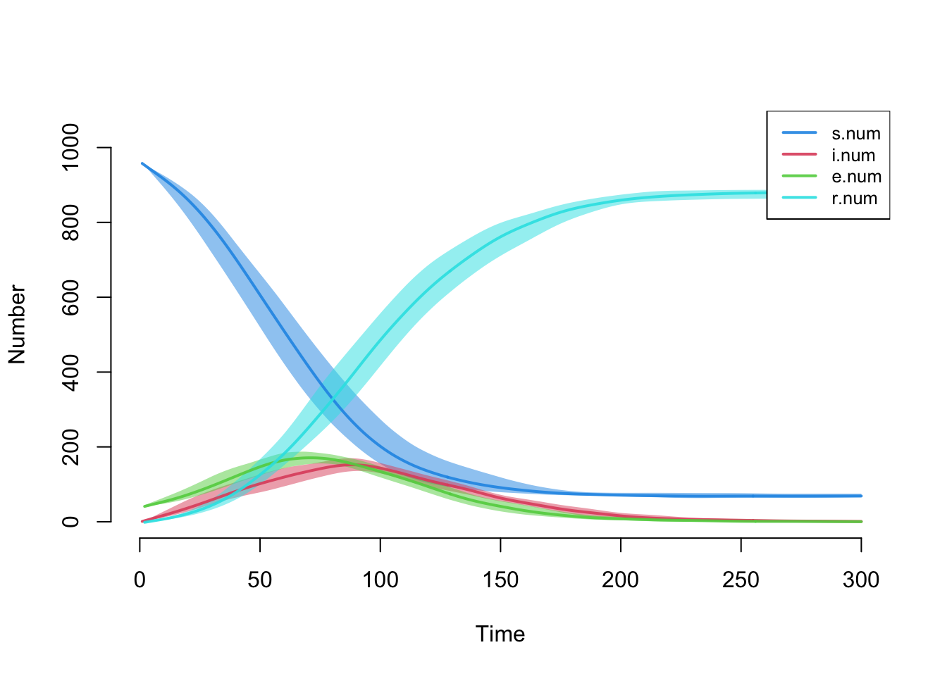
Here is a default plot of all the compartment sizes (all variables ending in .num), with the full quantile range set to 1.

Code

plot(sim, qnts = 1)

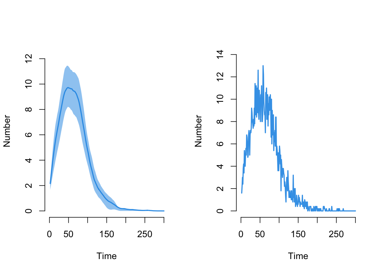
Here is the disease incidence, plotted in two ways:

Code

par(mfrow = c(1,2))
plot(sim, y = "se.flow")
plot(sim, y = "se.flow", mean.smooth = FALSE, qnts = FALSE)

Here is the new mean age summary statistic.

Code

par(mfrow = c(1,1))
plot(sim, y = "meanAge")

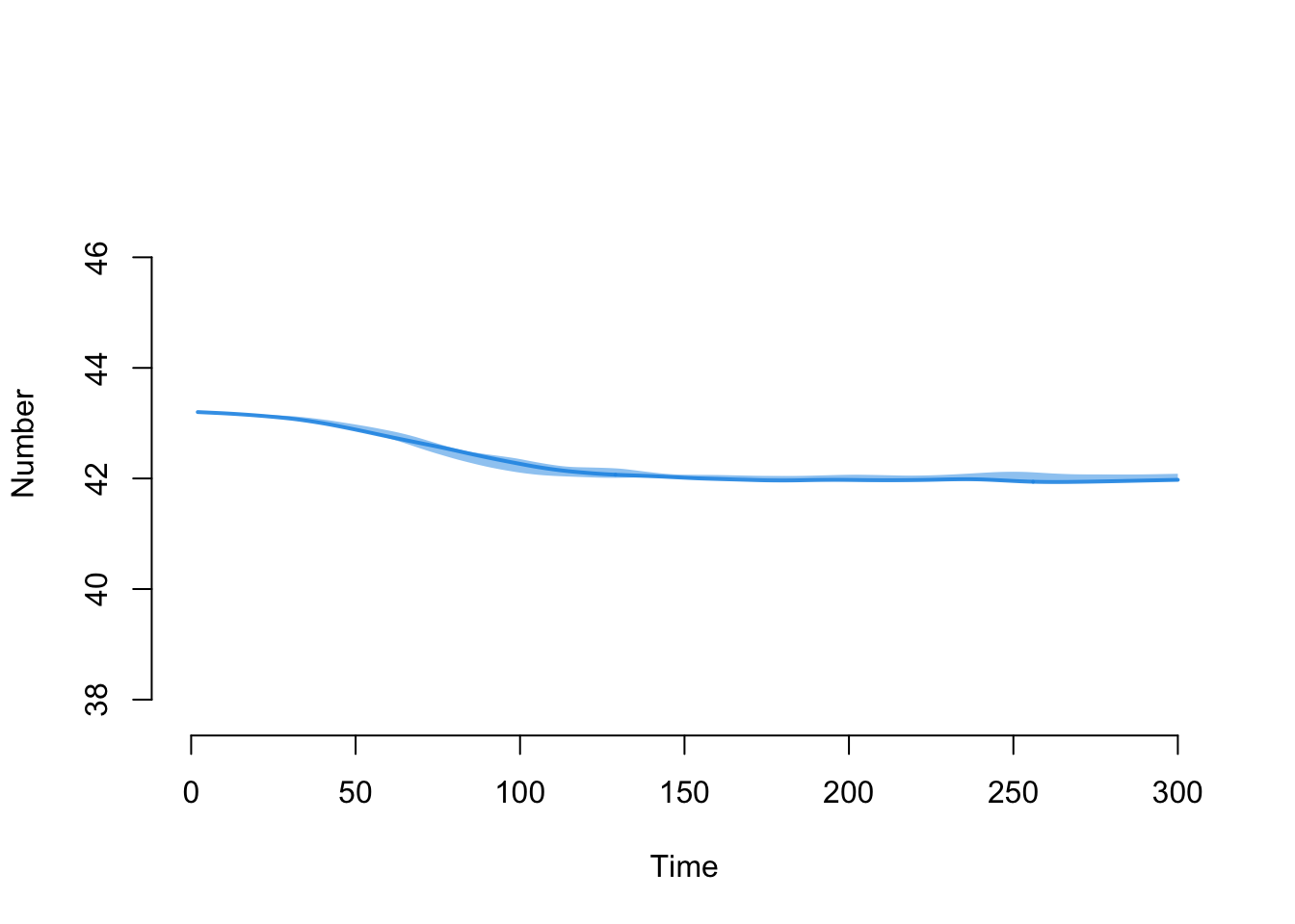
Let’s export the data into a data frame that averaged across the simulations and look at the starting and ending numerical values for mean age:

Code

df <- as.data.frame(sim, out = "mean")
head(df$meanAge)

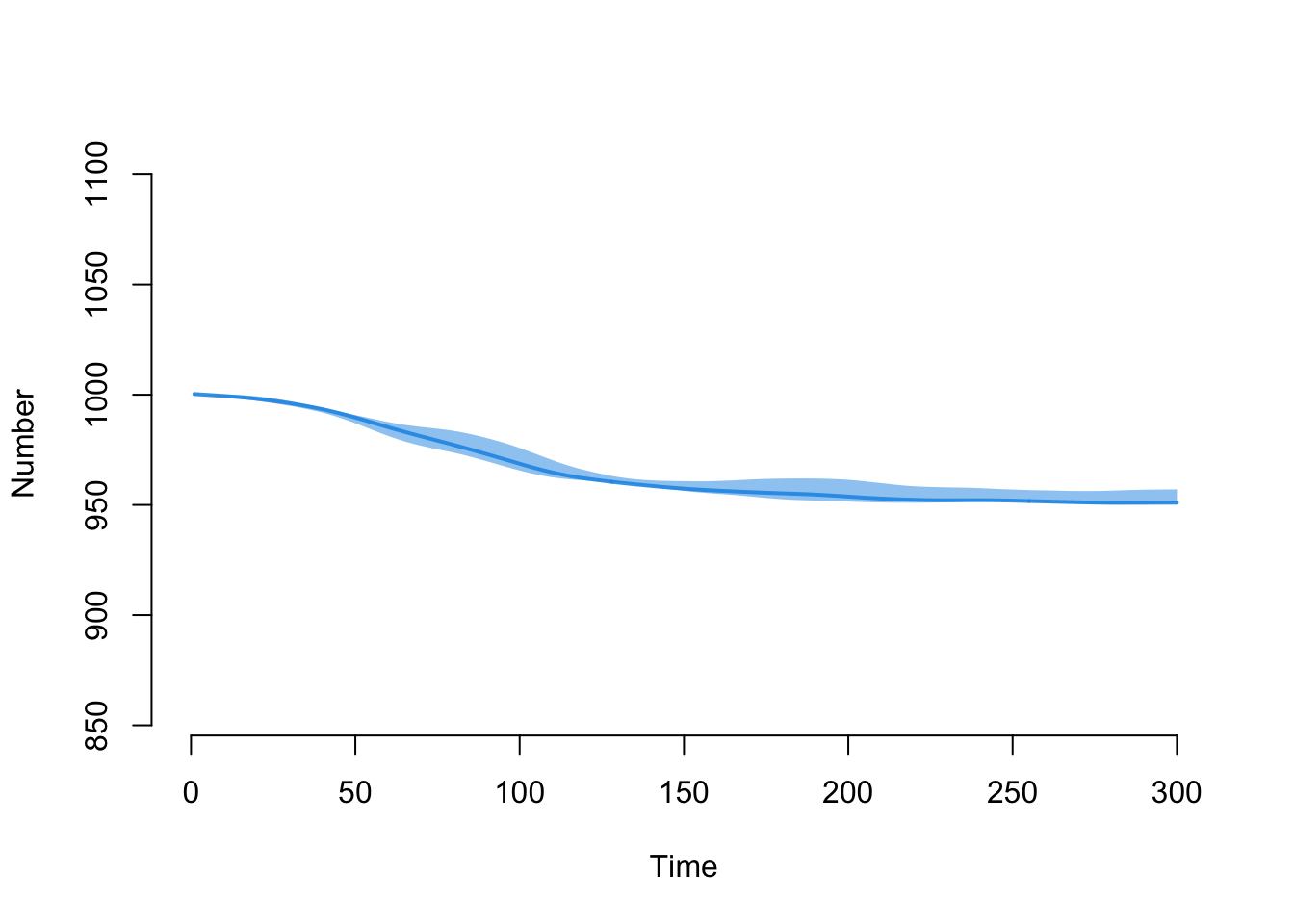
[1]      NaN 43.18374 43.18648 43.18922 43.19196 43.19470

Code

tail(df$meanAge)

[1] 41.96566 41.96840 41.97114 41.97388 41.97662 41.97936

Here is the decline in the overall population size over time:

Code

plot(sim, y = "num")

This plot shows the number of new total and COVID-related deaths each day.

Code

plot(sim, y = c("total.deaths", "covid.deaths"), qnts = FALSE, legend = TRUE)

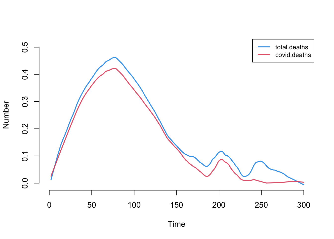
To demonstrate the transmission tree output for this extension model, we can extract the transmission matrix and then plot a phylogram:

Code

tm1 <- get_transmat(sim)
head(tm1, 20)

# A tibble: 20 × 6
# Groups:   at, sus [20]
      at   sus   inf transProb actRate finalProb
   <int> <int> <int>     <dbl>   <dbl>     <dbl>
 1     2    54   619       0.1       3     0.271
 2     3   193   469       0.1       3     0.271
 3     5   301   307       0.1       3     0.271
 4     5   704   371       0.1       3     0.271
 5     6   107   307       0.1       3     0.271
 6     6   169   307       0.1       3     0.271
 7     7    34    65       0.1       3     0.271
 8     7   874   326       0.1       3     0.271
 9     7   991   193       0.1       3     0.271
10     8     5   282       0.1       3     0.271
11     8    95    65       0.1       3     0.271
12     8   115   929       0.1       3     0.271
13     8   194   193       0.1       3     0.271
14     8   937   694       0.1       3     0.271
15     8   992   267       0.1       3     0.271
16     9    72   717       0.1       3     0.271
17     9    83   694       0.1       3     0.271
18     9   356   267       0.1       3     0.271
19     9   771   369       0.1       3     0.271
20    10   360   117       0.1       3     0.271

Code

# Plot the phylogram for the first seed
phylo.tm1 <- as.phylo.transmat(tm1)

found multiple trees, returning a list of 39phylo objects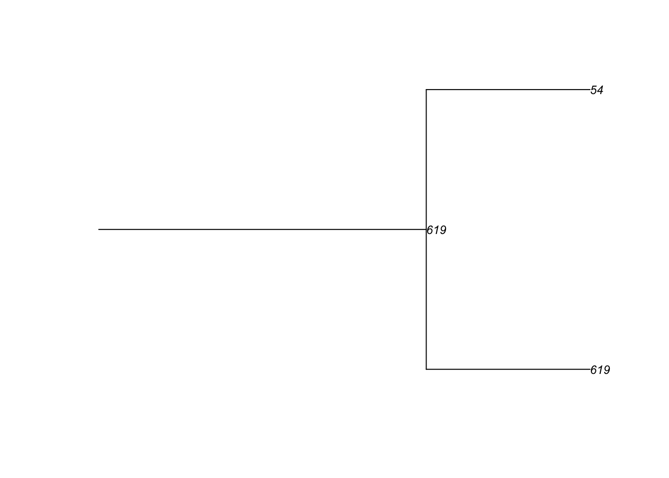

Code

plot(phylo.tm1[[1]], show.node.label = TRUE, root.edge = TRUE, cex = 0.75)

Overall, it appears that our new demographic features of the model are performing well!