SI Model with Age-Specific Vital Dynamics

vital dynamics

aging

beginner

An SI epidemic on a dynamic network with aging, births, and age-specific mortality using US life table data.

Author

Samuel M. Jenness

Published

August 1, 2018

Overview

This example demonstrates how to model an SI epidemic on a dynamic network with vital dynamics — aging, births (arrivals), and deaths (departures). In most real-world settings, populations are open: individuals are born, age, and die over the course of an epidemic. These demographic processes shape disease dynamics by continuously introducing new susceptibles (via births) and removing individuals (via death).

The key extension here is age-specific mortality using real US mortality data, combined with disease-induced excess mortality where infected individuals face a higher death rate. The network model also includes age-assortative mixing, so partnerships form preferentially between individuals close in age.

This is the foundational vital dynamics example in the Gallery. The three custom modules (aging, departures, arrivals) are building blocks reused and extended in many other examples.

Download standalone scripts

model.R — Main simulation script
module-fx.R — Custom module functions

Model Structure

Compartment	Label	Description
Susceptible	S	Not infected; at risk of infection through contact
Infectious	I	Infected and capable of transmitting (no recovery in SI)

flowchart LR
    in(( )) -->|"arrival<br/>(age 0)"| S
    S["<b>S</b><br/>Susceptible"] -->|"infection<br/>(si.flow)"| I["<b>I</b><br/>Infectious"]
    S -->|"age-specific<br/>mortality"| out1(( ))
    I -->|"age-specific ×<br/>disease multiplier"| out2(( ))

    style S fill:#3498db,color:#fff
    style I fill:#e74c3c,color:#fff
    style in fill:none,stroke:none
    style out1 fill:none,stroke:none
    style out2 fill:none,stroke:none

Three custom modules implement the demographic processes:

Aging: Each timestep represents one week. All nodes age by 1/52 years per step.
Departures (mortality): Age-specific weekly mortality from US life table data. Infected individuals have their rate multiplied by departure.disease.mult.
Arrivals (births): New susceptible nodes enter at age 0. The arrival rate is calibrated to the mean departure rate for approximate population stability.

Setup

suppressMessages(library(EpiModel))

nsims <- 5
ncores <- 5
nsteps <- 256

Vital Dynamics Data

Age-specific mortality rates from US population data, converted from per-100,000-per-year to per-person-per-week probabilities.

ages <- 0:85

# Age-specific mortality rates per 100,000 per year (US)
departure_rate <- c(588.45, 24.8, 11.7, 14.55, 47.85, 88.2, 105.65, 127.2,
                    154.3, 206.5, 309.3, 495.1, 736.85, 1051.15, 1483.45,
                    2294.15, 3642.95, 6139.4, 13938.3)

1dep_rate_pw <- departure_rate / 1e5 / 52

2age_spans <- c(1, 4, rep(5, 16), 1)
3dr_vec <- rep(dep_rate_pw, times = age_spans)

1: Convert from per-100,000-per-year to per-person-per-week (our timestep unit).
2: Age groups: 1 year for <1, 4 years for 1–4, then 5-year groups through 80–84, and 1 year for 85+.
3: Expand the 19 age-group rates into a vector of 86 yearly rates.

par(mar = c(3, 3, 2, 1), mgp = c(2, 1, 0))
barplot(dr_vec, col = "steelblue", border = NA,
        xlab = "Age", ylab = "Weekly Departure Rate",
        main = "Age-Specific Mortality Rates (US)")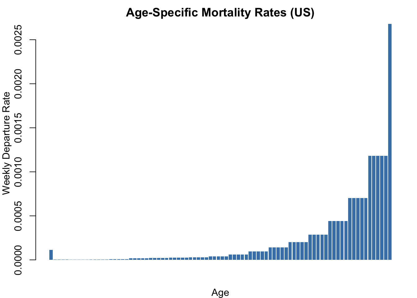

Figure 1: Age-specific weekly mortality rates derived from US life table data. Mortality is low from ages 1–40, then rises exponentially.

Custom Modules

Aging Module

Increments each node’s age by 1/52 per timestep and records the population mean age.

aging <- function(dat, at) {
  age <- get_attr(dat, "age")
1  age <- age + 1 / 52
  dat <- set_attr(dat, "age", age)

2  dat <- set_epi(dat, "meanAge", at, mean(age, na.rm = TRUE))

  return(dat)
}

1: One timestep = one week, so age increments by 1/52 of a year.
2: Track mean population age as an epidemiological summary statistic.

Departure Module

Simulates age-specific mortality with optional disease-induced excess mortality.

dfunc <- function(dat, at) {
  active <- get_attr(dat, "active")
  exitTime <- get_attr(dat, "exitTime")
  age <- get_attr(dat, "age")
  status <- get_attr(dat, "status")

  dep.rates <- get_param(dat, "departure.rates")
  dep.dis.mult <- get_param(dat, "departure.disease.mult")

  idsElig <- which(active == 1)
  nElig <- length(idsElig)
  nDepts <- 0

  if (nElig > 0) {
1    whole_ages_of_elig <- pmin(ceiling(age[idsElig]), 86)
    departure_rates_of_elig <- dep.rates[whole_ages_of_elig]

2    idsElig.inf <- which(status[idsElig] == "i")
    departure_rates_of_elig[idsElig.inf] <-
      departure_rates_of_elig[idsElig.inf] * dep.dis.mult

3    vecDepts <- which(rbinom(nElig, 1, departure_rates_of_elig) == 1)
    idsDepts <- idsElig[vecDepts]
    nDepts <- length(idsDepts)

    if (nDepts > 0) {
      active[idsDepts] <- 0
      exitTime[idsDepts] <- at
    }
  }

  dat <- set_attr(dat, "active", active)
  dat <- set_attr(dat, "exitTime", exitTime)
  dat <- set_epi(dat, "d.flow", at, nDepts)

  return(dat)
}

1: Map continuous age to the 86-element rate vector index. pmin(..., 86) caps ages 85+ at the final rate.
2: Infected individuals face excess mortality: their rate is multiplied by the disease multiplier parameter.
3: Bernoulli trial: each eligible node departs with their age-specific (and disease-adjusted) probability.

Arrival Module

Simulates births as new susceptible nodes entering at age 0.

afunc <- function(dat, at) {
  n <- sum(get_attr(dat, "active") == 1)
  a.rate <- get_param(dat, "arrival.rate")

  nArrivalsExp <- n * a.rate
1  nArrivals <- rpois(1, nArrivalsExp)

  if (nArrivals > 0) {
2    dat <- append_core_attr(dat, at, nArrivals)
    dat <- append_attr(dat, "status", "s", nArrivals)
    dat <- append_attr(dat, "infTime", NA, nArrivals)
3    dat <- append_attr(dat, "age", 0, nArrivals)
  }

  dat <- set_epi(dat, "a.flow", at, nArrivals)

  return(dat)
}

1: Number of births is Poisson-distributed, scaled by current population size.
2: append_core_attr() initializes required node attributes (active status, unique ID, etc.).
3: All newborns enter at age 0 as susceptibles.

Network Model

n <- 500
nw <- network_initialize(n)

ageVec <- sample(ages, n, replace = TRUE)
nw <- set_vertex_attribute(nw, "age", ageVec)

# Formation: edges + age-assortative mixing
1formation <- ~edges + absdiff("age")

mean_degree <- 0.8
n_edges <- mean_degree * (n / 2)
avg.abs.age.diff <- 1.5
2target.stats <- c(n_edges, n_edges * avg.abs.age.diff)

# Dissolution: adjust for population turnover
coef.diss <- dissolution_coefs(~offset(edges), duration = 60,
3                               d.rate = mean(dr_vec))
coef.diss

est <- netest(nw, formation, target.stats, coef.diss)

1: absdiff("age") controls age-assortative mixing — partners tend to be close in age.
2: Target: mean degree of 0.8 with average absolute age difference of 1.5 years within partnerships.
3: The d.rate argument adjusts dissolution coefficients for population turnover so observed partnership duration matches the intended 60 weeks.

Dissolution Coefficients
=======================
Dissolution Model: ~offset(edges)
Target Statistics: 60
Crude Coefficient: 4.077537
Mortality/Exit Rate: 0.0002217519
Adjusted Coefficient: 4.104505

Network Diagnostics

dx <- netdx(est, nsims = nsims, ncores = ncores, nsteps = nsteps,
            nwstats.formula = ~edges + absdiff("age") + isolates + degree(0:5))


Network Diagnostics
-----------------------
- Simulating 5 networks
- Calculating formation statistics

print(dx)

EpiModel Network Diagnostics
=======================
Diagnostic Method: Dynamic
Simulations: 5
Time Steps per Sim: 256

Formation Diagnostics
----------------------- 
            Target Sim Mean Pct Diff Sim SE Z Score SD(Sim Means) SD(Statistic)
edges          200  194.680   -2.660  2.166  -2.456         3.981        11.402
absdiff.age    300  296.666   -1.111  5.783  -0.577         9.377        28.368
isolates        NA  230.510       NA  2.399      NA         5.695        12.771
degree0         NA  230.510       NA  2.399      NA         5.695        12.771
degree1         NA  176.392       NA  1.778      NA         4.471        11.375
degree2         NA   70.998       NA  1.180      NA         1.888         7.961
degree3         NA   17.926       NA  0.452      NA         0.783         3.662
degree4         NA    3.713       NA  0.220      NA         0.308         1.912
degree5         NA    0.423       NA  0.069      NA         0.118         0.643

Duration Diagnostics
----------------------- 
      Target Sim Mean Pct Diff Sim SE Z Score SD(Sim Means) SD(Statistic)
edges     60   58.585   -2.358  0.703  -2.012         2.082          3.95

Dissolution Diagnostics
----------------------- 
      Target Sim Mean Pct Diff Sim SE Z Score SD(Sim Means) SD(Statistic)
edges  0.017    0.017    2.571      0   1.718         0.001         0.009

plot(dx)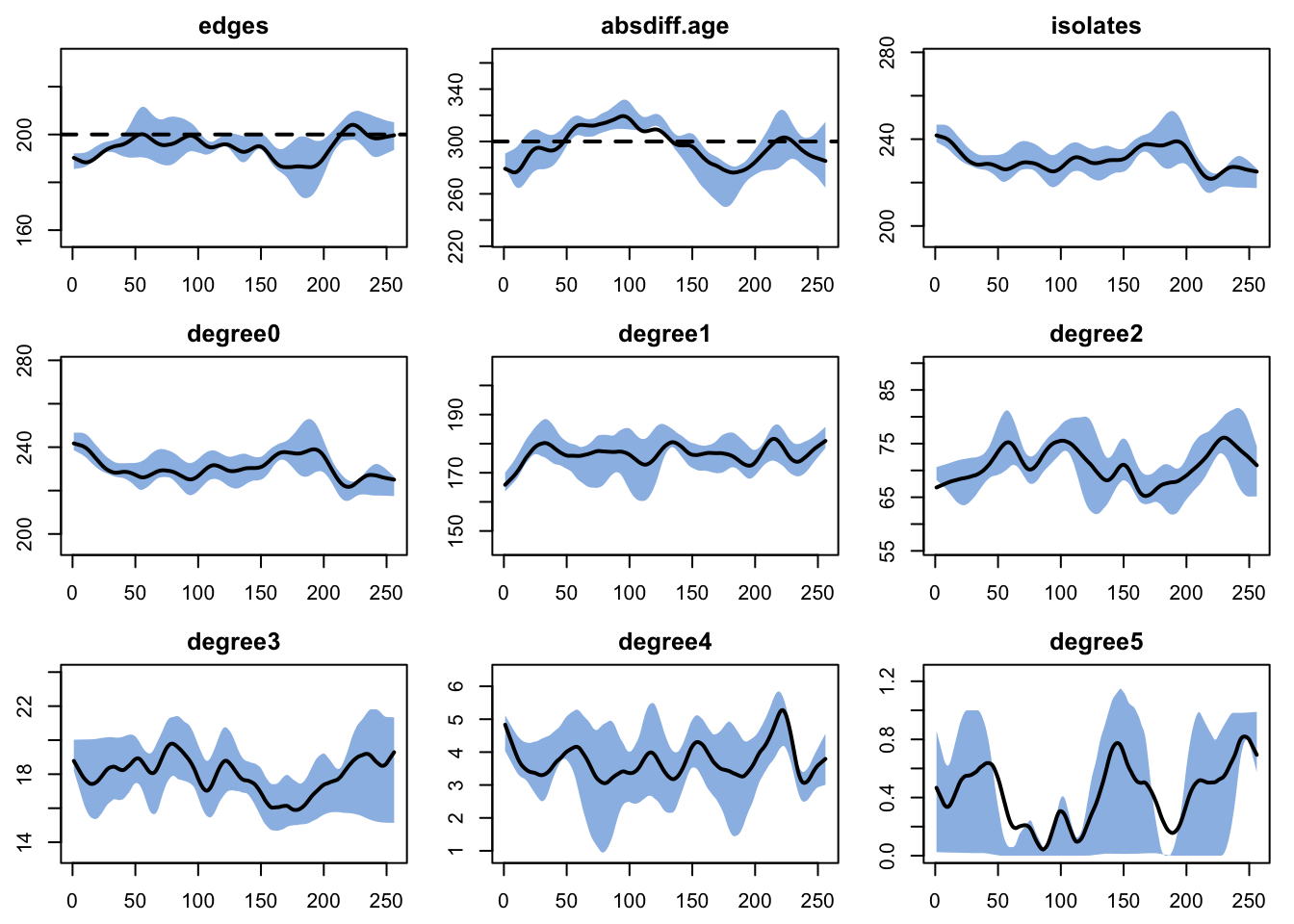

Figure 2: Network diagnostic plots verifying the simulation reproduces target statistics.

Epidemic Simulation

Scenario 1: No Disease-Induced Mortality (Baseline)

All-cause mortality only. Disease has no effect on survival, so the population size remains stable and prevalence rises toward saturation.

init <- init.net(i.num = 50)

param_base <- param.net(
  inf.prob = 0.15,
  departure.rates = dr_vec,
1  departure.disease.mult = 1,
  arrival.rate = mean(dr_vec)
)

control <- control.net(
2  type = NULL,
  nsims = nsims,
  ncores = ncores,
  nsteps = nsteps,
  aging.FUN = aging,
  departures.FUN = dfunc,
  arrivals.FUN = afunc,
  infection.FUN = infection.net,
  resim_nets.FUN = resim_nets,
3  resimulate.network = TRUE,
  verbose = FALSE
)

sim_base <- netsim(est, param_base, init, control)
print(sim_base)

1: Multiplier of 1 = disease has no effect on mortality.
2: type = NULL means all modules are custom (no built-in SIS/SIR logic).
3: Network must be resimulated each step because ages change and the ERGM formation model includes absdiff("age").

EpiModel Simulation
=======================
Model class: netsim

Simulation Summary
-----------------------
Model type:
No. simulations: 5
No. time steps: 256
No. NW groups: 1

Fixed Parameters
---------------------------
inf.prob = 0.15
departure.rates = 0.0001131635 4.769231e-06 4.769231e-06 4.769231e-06 
4.769231e-06 2.25e-06 2.25e-06 2.25e-06 2.25e-06 2.25e-06 ...
departure.disease.mult = 1
arrival.rate = 0.0002217519
act.rate = 1
groups = 1

Model Functions
-----------------------
initialize.FUN 
resim_nets.FUN 
summary_nets.FUN 
infection.FUN 
departures.FUN 
arrivals.FUN 
nwupdate.FUN 
prevalence.FUN 
verbose.FUN 
aging.FUN 

Model Output
-----------------------
Variables: s.num i.num num meanAge si.flow d.flow a.flow
Networks: sim1 ... sim5
Transmissions: sim1 ... sim5

Formation Statistics
----------------------- 
            Target Sim Mean Pct Diff Sim SE Z Score SD(Sim Means) SD(Statistic)
edges          200  200.079    0.039  2.631   0.030         6.601        13.035
absdiff.age    300  288.584   -3.805  5.645  -2.022        20.211        29.951


Duration Statistics
----------------------- 
      Target Sim Mean Pct Diff Sim SE Z Score SD(Sim Means) SD(Statistic)
edges     60   61.287    2.145  0.511    2.52         1.201         2.936

Dissolution Statistics
----------------------- 
      Target Sim Mean Pct Diff Sim SE Z Score SD(Sim Means) SD(Statistic)
edges  0.017    0.016   -1.673      0  -1.109             0         0.009

Scenario 2: Disease-Induced Mortality (50x)

Infected individuals face 50x the baseline age-specific mortality rate — exaggerated for pedagogical clarity.

param_lethal <- param.net(
  inf.prob = 0.15,
  departure.rates = dr_vec,
  departure.disease.mult = 50,
  arrival.rate = mean(dr_vec)
)

sim_lethal <- netsim(est, param_lethal, init, control)
print(sim_lethal)

EpiModel Simulation
=======================
Model class: netsim

Simulation Summary
-----------------------
Model type:
No. simulations: 5
No. time steps: 256
No. NW groups: 1

Fixed Parameters
---------------------------
inf.prob = 0.15
departure.rates = 0.0001131635 4.769231e-06 4.769231e-06 4.769231e-06 
4.769231e-06 2.25e-06 2.25e-06 2.25e-06 2.25e-06 2.25e-06 ...
departure.disease.mult = 50
arrival.rate = 0.0002217519
act.rate = 1
groups = 1

Model Functions
-----------------------
initialize.FUN 
resim_nets.FUN 
summary_nets.FUN 
infection.FUN 
departures.FUN 
arrivals.FUN 
nwupdate.FUN 
prevalence.FUN 
verbose.FUN 
aging.FUN 

Model Output
-----------------------
Variables: s.num i.num num meanAge si.flow d.flow a.flow
Networks: sim1 ... sim5
Transmissions: sim1 ... sim5

Formation Statistics
----------------------- 
            Target Sim Mean Pct Diff Sim SE Z Score SD(Sim Means) SD(Statistic)
edges          200  159.886  -20.057   5.66  -7.088         8.029        20.224
absdiff.age    300  245.053  -18.316   8.07  -6.809         9.163        32.691


Duration Statistics
----------------------- 
      Target Sim Mean Pct Diff Sim SE Z Score SD(Sim Means) SD(Statistic)
edges     60   57.488   -4.187  0.644  -3.899         0.824         3.591

Dissolution Statistics
----------------------- 
      Target Sim Mean Pct Diff Sim SE Z Score SD(Sim Means) SD(Statistic)
edges  0.017    0.019   13.745      0   7.077             0         0.011

Analysis

sim_base <- mutate_epi(sim_base, prev = i.num / num)
sim_lethal <- mutate_epi(sim_lethal, prev = i.num / num)

Prevalence Comparison

Without disease mortality, SI prevalence saturates near 1 as everyone eventually becomes infected. With lethal disease, mortality removes infected individuals before they can transmit, slowing the epidemic.

par(mfrow = c(1, 1), mar = c(3, 3, 2, 1), mgp = c(2, 1, 0))
plot(sim_base, y = "prev",
     main = "Prevalence: Baseline vs. Disease Mortality",
     ylab = "Prevalence (I / N)", xlab = "Week",
     mean.col = "steelblue", mean.lwd = 2, mean.smooth = TRUE,
     qnts.col = "steelblue", qnts.alpha = 0.2, qnts.smooth = TRUE,
     legend = FALSE)
plot(sim_lethal, y = "prev",
     mean.col = "firebrick", mean.lwd = 2, mean.smooth = TRUE,
     qnts.col = "firebrick", qnts.alpha = 0.2, qnts.smooth = TRUE,
     legend = FALSE, add = TRUE)
legend("topleft", legend = c("Baseline (mult=1)", "Lethal (mult=50)"),
       col = c("steelblue", "firebrick"), lwd = 2, bty = "n")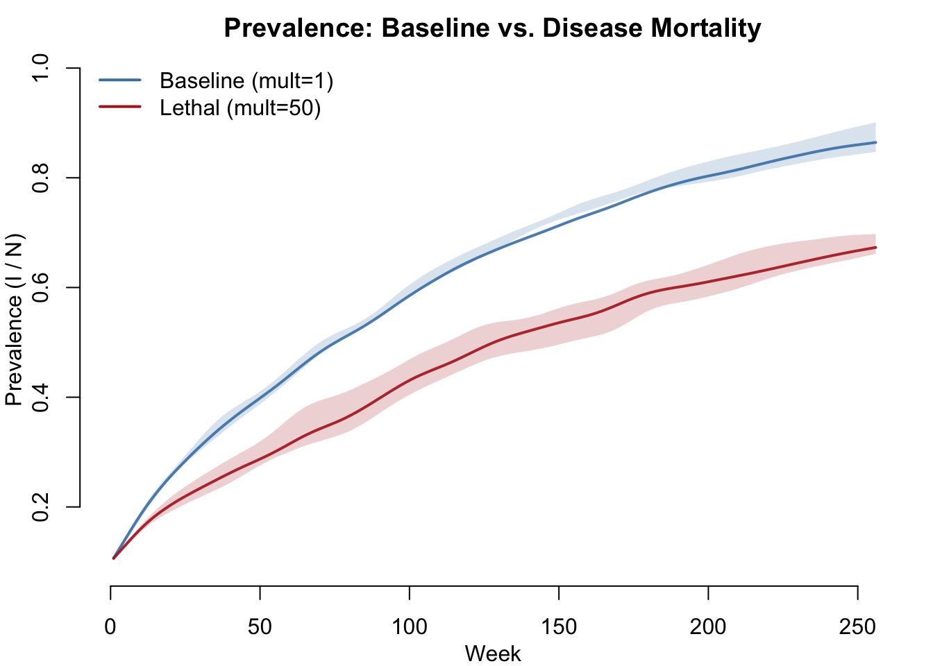

Figure 3: Prevalence over time. Blue: baseline (no disease mortality). Red: 50x disease-induced mortality.

Population Size

Baseline: population stable (arrivals approximately equal departures). Lethal: population declines because disease-induced mortality exceeds the birth rate calibrated to background mortality only.

par(mfrow = c(1, 1), mar = c(3, 3, 2, 1), mgp = c(2, 1, 0))
plot(sim_base, y = "num",
     main = "Population Size",
     ylab = "Total Population", xlab = "Week",
     mean.col = "steelblue", mean.lwd = 2, mean.smooth = TRUE,
     qnts.col = "steelblue", qnts.alpha = 0.2, qnts.smooth = TRUE,
     ylim = c(200, 600), legend = FALSE)
plot(sim_lethal, y = "num",
     mean.col = "firebrick", mean.lwd = 2, mean.smooth = TRUE,
     qnts.col = "firebrick", qnts.alpha = 0.2, qnts.smooth = TRUE,
     legend = FALSE, add = TRUE)
legend("topright", legend = c("Baseline (mult=1)", "Lethal (mult=50)"),
       col = c("steelblue", "firebrick"), lwd = 2, bty = "n")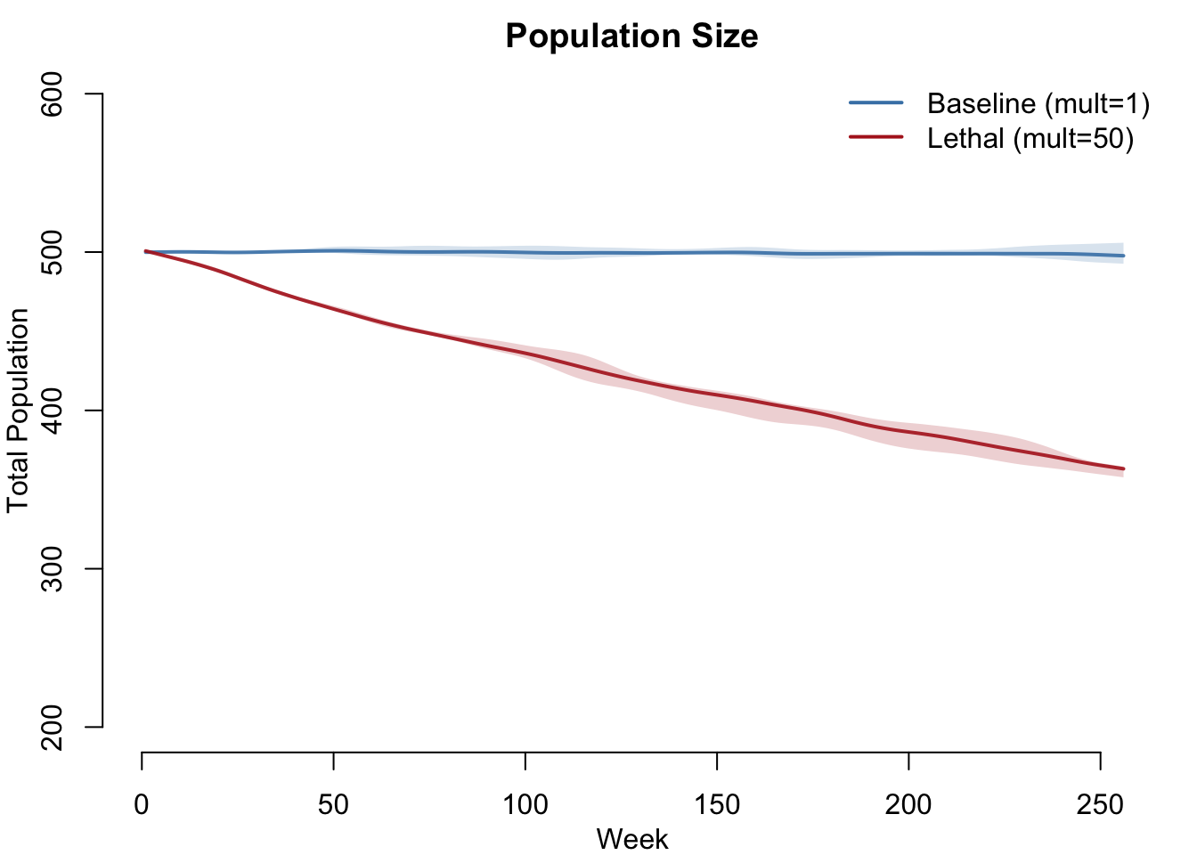

Figure 4: Total population over time under baseline and lethal disease scenarios.

Vital Dynamics Detail (Lethal Scenario)

par(mfrow = c(2, 2), mar = c(3, 3, 2, 1), mgp = c(2, 1, 0))

plot(sim_lethal, y = "meanAge",
     main = "Mean Age", ylab = "Years", xlab = "Week",
     mean.col = "firebrick", mean.lwd = 2, mean.smooth = TRUE,
     qnts.col = "firebrick", qnts.alpha = 0.2, qnts.smooth = TRUE,
     legend = FALSE)

plot(sim_lethal, y = "d.flow",
     main = "Departures per Week", ylab = "Count", xlab = "Week",
     mean.col = "firebrick", mean.lwd = 2, mean.smooth = TRUE,
     qnts.col = "firebrick", qnts.alpha = 0.2, qnts.smooth = TRUE,
     legend = FALSE)

plot(sim_lethal, y = "a.flow",
     main = "Arrivals per Week", ylab = "Count", xlab = "Week",
     mean.col = "#27ae60", mean.lwd = 2, mean.smooth = TRUE,
     qnts.col = "#27ae60", qnts.alpha = 0.2, qnts.smooth = TRUE,
     legend = FALSE)

plot(sim_lethal, y = "s.num",
     main = "Susceptible Count", ylab = "Count", xlab = "Week",
     mean.col = "steelblue", mean.lwd = 2, mean.smooth = TRUE,
     qnts.col = "steelblue", qnts.alpha = 0.2, qnts.smooth = TRUE,
     legend = FALSE)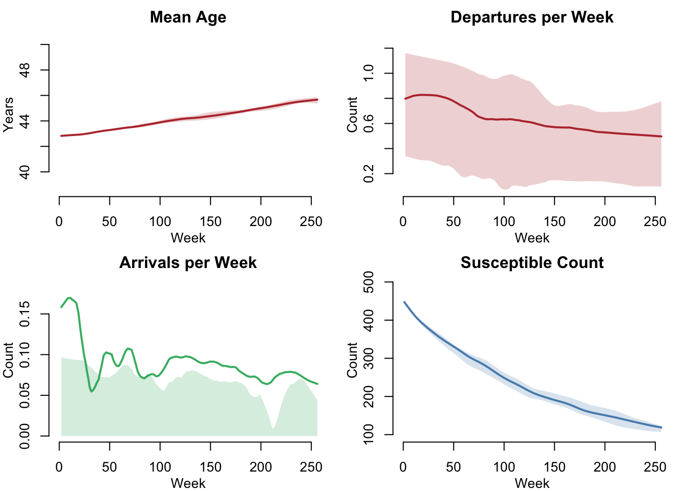

Figure 5: Four-panel view of the lethal disease scenario showing demographic impacts.

New Infections

par(mfrow = c(1, 1), mar = c(3, 3, 2, 1), mgp = c(2, 1, 0))
plot(sim_base, y = "si.flow",
     main = "New Infections: Baseline vs. Disease Mortality",
     ylab = "New Infections per Week", xlab = "Week",
     mean.col = "steelblue", mean.lwd = 2, mean.smooth = TRUE,
     qnts.col = "steelblue", qnts.alpha = 0.2, qnts.smooth = TRUE,
     legend = FALSE)
plot(sim_lethal, y = "si.flow",
     mean.col = "firebrick", mean.lwd = 2, mean.smooth = TRUE,
     qnts.col = "firebrick", qnts.alpha = 0.2, qnts.smooth = TRUE,
     legend = FALSE, add = TRUE)
legend("topright", legend = c("Baseline (mult=1)", "Lethal (mult=50)"),
       col = c("steelblue", "firebrick"), lwd = 2, bty = "n")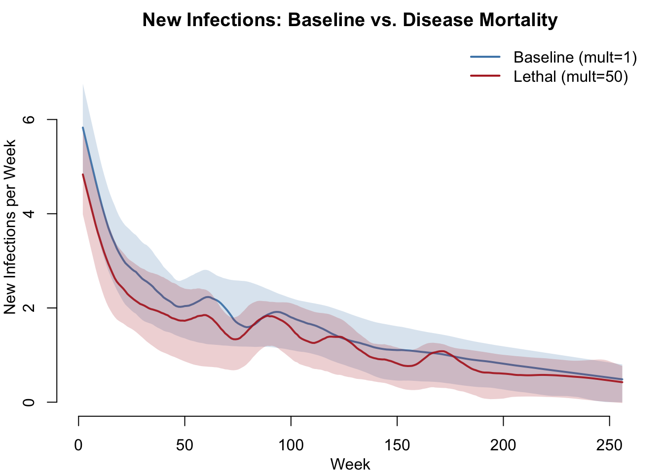

Summary Table

df_base <- as.data.frame(sim_base)
df_lethal <- as.data.frame(sim_lethal)

knitr::kable(data.frame(
  Metric = c("Mean prevalence",
             "Final prevalence",
             "Mean population size",
             "Final population size",
             "Cumulative departures",
             "Cumulative infections"),
  Baseline = c(
    round(mean(df_base$prev, na.rm = TRUE), 3),
    round(mean(df_base$prev[df_base$time == max(df_base$time)], na.rm = TRUE), 3),
    round(mean(df_base$num, na.rm = TRUE)),
    round(mean(df_base$num[df_base$time == max(df_base$time)], na.rm = TRUE)),
    round(mean(tapply(df_base$d.flow, df_base$sim, sum, na.rm = TRUE))),
    round(mean(tapply(df_base$si.flow, df_base$sim, sum, na.rm = TRUE)))
  ),
  Lethal = c(
    round(mean(df_lethal$prev, na.rm = TRUE), 3),
    round(mean(df_lethal$prev[df_lethal$time == max(df_lethal$time)], na.rm = TRUE), 3),
    round(mean(df_lethal$num, na.rm = TRUE)),
    round(mean(df_lethal$num[df_lethal$time == max(df_lethal$time)], na.rm = TRUE)),
    round(mean(tapply(df_lethal$d.flow, df_lethal$sim, sum, na.rm = TRUE))),
    round(mean(tapply(df_lethal$si.flow, df_lethal$sim, sum, na.rm = TRUE)))
  )
))

Table 1

Metric	Baseline	Lethal
Mean prevalence	0.612	0.461
Final prevalence	0.865	0.674
Mean population size	500.000	424.000
Final population size	497.000	363.000
Cumulative departures	33.000	161.000
Cumulative infections	401.000	336.000

Parameters

Transmission

Parameter	Description	Default
`inf.prob`	Per-act transmission probability	0.15
`act.rate`	Acts per partnership per week (built-in default)	1

Vital Dynamics

Parameter	Description	Default
`departure.rates`	Age-specific weekly mortality rates (86-element vector)	US life table data
`departure.disease.mult`	Multiplier on departure rates for infected individuals	1 (baseline) or 50 (lethal)
`arrival.rate`	Per-capita weekly birth rate	`mean(departure.rates)`

Network

Parameter	Description	Default
Population size	Number of nodes	500
Mean degree	Average concurrent partnerships per node	0.8
Age assortativity	Mean absolute age difference within partnerships	1.5 years
Partnership duration	Mean edge duration (weeks)	60 (~1.2 years)

Module Execution Order

aging → departures (dfunc) → arrivals (afunc) → resim_nets → infection → prevalence

Aging runs first so that departure rates reflect updated ages. Arrivals follow departures to replace the departed. Network resimulation happens after demographic changes so the ERGM respects the new population composition. Infection then runs on the updated network.

Next Steps

Add disease recovery to convert this SI model to an SIS or SIR model — see Adding an Exposed State for the progression module pattern
Use more granular age categories or empirical life table data for country-specific mortality
Add heterogeneous susceptibility that varies by age
Add stage-dependent infectiousness and mortality — see the HIV model for disease stage–specific departure rates