flowchart TD
    S["<b>S</b><br/>Susceptible"] -->|"infection by strain 1<br/>(si.flow)"| I1["<b>I1</b><br/>Strain 1 (acute)<br/>inf.prob = 0.5"]
    S -->|"infection by strain 2<br/>(si.flow.st2)"| I2["<b>I2</b><br/>Strain 2 (chronic)<br/>inf.prob.st2 = 0.01"]
    I1 -->|"fast recovery<br/>(rec.rate = 0.05)"| S
    I2 -->|"slow recovery<br/>(rec.rate.st2 = 0.005)"| S

    style S fill:#3498db,color:#fff
    style I1 fill:#e74c3c,color:#fff
    style I2 fill:#2980b9,color:#fff
Competing Pathogen Strains in an SIS Epidemic
SIS
multi-strain
network effects
intermediate
Models SIS with two competing strains differing in transmission-duration trade-offs, showing how network concurrency determines which strain dominates.
Overview
This example models an SIS epidemic with two competing pathogen strains that differ in their transmission strategy: one is highly infectious but short-lived (an “acute” strain), while the other has low infectiousness but persists for much longer (a “chronic” strain). This trade-off between infectiousness and duration is common in real pathogens — for example, gonorrhea vs. chlamydia, or different variants of the same pathogen.
The central question: which transmission strategy wins? The answer depends critically on the network structure — specifically, whether concurrency (simultaneous partnerships) is allowed. Concurrency amplifies transmission by allowing an infected individual to spread the pathogen to a new partner before the existing partnership ends, creating branching chains of transmission. This benefits the fast-spreading acute strain disproportionately.
This example demonstrates how to extend EpiModel’s infection and recovery modules to track multiple strains, and how network structure (not just individual-level parameters) can determine epidemic outcomes.
TipDownload standalone scripts
- model.R — Main simulation script
- module-fx.R — Custom module functions
Model Structure
| Compartment | Label | Description |
|---|---|---|
| Susceptible | S | Not infected; at risk of infection by either strain |
| Infectious (Strain 1) | I1 | Infected with the acute strain (high transmission, fast recovery) |
| Infectious (Strain 2) | I2 | Infected with the chronic strain (low transmission, slow recovery) |
This is an SIS model — recovered individuals return to the susceptible pool and can be reinfected by either strain. The two strains compete for the same pool of susceptible hosts. Key dynamics:
- Competitive exclusion: In many parameter regimes, one strain dominates and drives the other to extinction. The strains compete indirectly — by infecting susceptibles, each strain reduces the pool available to the other.
- Coexistence is possible at intermediate concurrency levels, where both strains maintain endemic equilibria simultaneously.
- No co-infection: An individual can only be infected with one strain at a time. On recovery, they become fully susceptible to both strains again.
- Strain inheritance: Newly infected individuals inherit the strain of their infecting partner. There is no mutation or recombination.
Why Concurrency Matters
The two network models have identical mean degree, partnership duration, and act rates. The only difference is whether concurrency is allowed. Yet this structural difference reverses which strain dominates:
- With concurrency: The acute strain (high
inf.prob, fast recovery) can exploit branching transmission chains. An infected individual with 2+ partners can transmit to a new partner before recovering, even with a short infectious period. The fast transmission rate dominates. - Without concurrency (monogamy): Partners are sequential. The acute strain’s high per-act probability provides little advantage because transmission to each new partner must wait for the previous partnership to dissolve. The chronic strain’s long infectious duration means it persists across multiple sequential partnerships, giving it the advantage.
Setup
suppressMessages(library(EpiModel))

nsims <- 5
ncores <- 5
nsteps <- 500
Custom Modules
Strain Initialization Module
Runs once at the first module call (timestep 2). Each initially infected node is randomly assigned to strain 1 or strain 2 via a Bernoulli draw, with the probability of strain 2 controlled by pct.st2. Susceptible nodes receive NA for their strain attribute.
init_strain <- function(dat, at) {

1  if (is.null(get_attr(dat, "strain", override.null.error = TRUE))) {

    active <- get_attr(dat, "active")
    status <- get_attr(dat, "status")

    nActive <- sum(active == 1)
    idsInf <- which(active == 1 & status == "i")

    pct.st2 <- get_param(dat, "pct.st2")

2    strain <- rep(NA, nActive)
3    strain[idsInf] <- rbinom(length(idsInf), 1, pct.st2) + 1

    dat <- set_attr(dat, "strain", strain)
  }

  return(dat)
}- 1
-
override.null.error = TRUEreturnsNULLinstead of erroring when the attribute does not exist, allowing a one-time initialization check. - 2
-
Susceptible nodes have
NAfor strain — they carry no pathogen. - 3
-
rbinom(..., 1, pct.st2) + 1produces 1 or 2: strain 1 with probability1 - pct.st2, strain 2 with probabilitypct.st2.
Two-Strain Infection Module
Replaces EpiModel’s built-in infection.net to implement strain-specific transmission. For each discordant edge, the per-act transmission probability depends on the infected partner’s strain. Newly infected individuals inherit the infecting partner’s strain.
infection.2strains <- function(dat, at) {

  ## Attributes ##
  active <- get_attr(dat, "active")
  status <- get_attr(dat, "status")
  infTime <- get_attr(dat, "infTime")
  strain <- get_attr(dat, "strain")

  ## Parameters ##
  inf.prob <- get_param(dat, "inf.prob")
  act.rate <- get_param(dat, "act.rate")
  inf.prob.st2 <- get_param(dat, "inf.prob.st2")

  ## Eligible nodes ##
  idsInf <- which(active == 1 & status == "i")
  nActive <- sum(active == 1)
  nElig <- length(idsInf)

  ## Initialize flow counters ##
  nInf <- nInfST2 <- totInf <- 0

  if (nElig > 0 && nElig < nActive) {

1    del <- discord_edgelist(dat, at)

    if (!(is.null(del))) {

      del$infDur <- at - infTime[del$inf]
      del$infDur[del$infDur == 0] <- 1

      # Strain-specific transmission probabilities
      linf.prob <- length(inf.prob)
      linf.prob.st2 <- length(inf.prob.st2)

2      del$transProb <- ifelse(strain[del$inf] == 1,
                              ifelse(del$infDur <= linf.prob,
                                     inf.prob[del$infDur],
                                     inf.prob[linf.prob]),
                              ifelse(del$infDur <= linf.prob.st2,
                                     inf.prob.st2[del$infDur],
                                     inf.prob.st2[linf.prob.st2]))

      # Optional intervention effect
      if (!is.null(dat$param$inter.eff) && at >= dat$param$inter.start) {
        del$transProb <- del$transProb * (1 - dat$param$inter.eff)
      }

      lact.rate <- length(act.rate)
      del$actRate <- ifelse(del$infDur <= lact.rate,
                            act.rate[del$infDur],
                            act.rate[lact.rate])

3      del$finalProb <- 1 - (1 - del$transProb) ^ del$actRate

      transmit <- rbinom(nrow(del), 1, del$finalProb)
      del <- del[which(transmit == 1), ]

      idsNewInf <- unique(del$sus)

      # Resolve double infections: first infector determines strain
4      infpairs <- sapply(idsNewInf, function(x) min(which(del$sus == x)))

      if (length(infpairs) > 0) {
        infectors <- del$inf[infpairs]
        strain <- get_attr(dat, "strain")
        infectors_strain <- strain[infectors]

        nInf <- sum(infectors_strain == 1)
        nInfST2 <- sum(infectors_strain == 2)
        totInf <- nInf + nInfST2
      } else {
        nInf <- nInfST2 <- totInf <- 0
      }

      ## Update attributes for newly infected ##
      if (totInf > 0) {
        status[idsNewInf] <- "i"
        dat <- set_attr(dat, "status", status)
        infTime[idsNewInf] <- at
        dat <- set_attr(dat, "infTime", infTime)
5        strain[idsNewInf] <- strain[infectors]
        dat <- set_attr(dat, "strain", strain)
      }

    }
  }

  ## Summary statistics ##
  dat <- set_epi(dat, "si.flow", at, nInf)
  dat <- set_epi(dat, "si.flow.st2", at, nInfST2)
  dat <- set_epi(dat, "i.num.st1", at, sum(status == "i" & strain == 1))
  dat <- set_epi(dat, "i.num.st2", at, sum(status == "i" & strain == 2))

  return(dat)
}- 1
-
discord_edgelist()returns all edges between susceptible and infected nodes — the potential transmission events. - 2
-
Transmission probability is looked up by the infector’s strain. Both
inf.probandinf.prob.st2can be vectors indexed by infection duration, allowing time-varying infectiousness. - 3
-
Per-timestep probability accounts for multiple acts:
P(transmit) = 1 - (1 - p)^acts. - 4
- When a susceptible has discordant edges with multiple infected partners and multiple transmissions occur, the first infector (by edgelist row order) determines the strain.
- 5
- Newly infected individuals inherit the strain of their infecting partner — no mutation or recombination.
Two-Strain Recovery Module
Replaces EpiModel’s built-in recovery module to implement strain-dependent recovery rates. Strain 1 recovers at rec.rate (fast), strain 2 at rec.rate.st2 (slow). On recovery, both disease status and strain assignment are cleared.
recov.2strains <- function(dat, at) {

  ## Attributes ##
  active <- get_attr(dat, "active")
  status <- get_attr(dat, "status")
  strain <- get_attr(dat, "strain")

  ## Parameters ##
  rec.rate <- get_param(dat, "rec.rate")
  rec.rate.st2 <- get_param(dat, "rec.rate.st2")

  ## Determine eligible to recover ##
  idsElig <- which(active == 1 & status == "i")
  nElig <- length(idsElig)

  ## Strain-dependent recovery rates ##
  strain.elig <- strain[idsElig]
1  ratesElig <- ifelse(strain.elig == 1, rec.rate, rec.rate.st2)

  ## Stochastic recovery ##
2  vecRecov <- which(rbinom(nElig, 1, ratesElig) == 1)
  idsRecov <- idsElig[vecRecov]
  nRecov <- length(idsRecov)
  nRecov.st1 <- sum(strain[idsRecov] == 1)
  nRecov.st2 <- sum(strain[idsRecov] == 2)

  ## Update attributes for recovered individuals ##
  status[idsRecov] <- "s"
3  strain[idsRecov] <- NA

  dat <- set_attr(dat, "status", status)
  dat <- set_attr(dat, "strain", strain)

  ## Summary statistics ##
  dat <- set_epi(dat, "is.flow", at, nRecov)
  dat <- set_epi(dat, "is.flow.st1", at, nRecov.st1)
  dat <- set_epi(dat, "is.flow.st2", at, nRecov.st2)

  return(dat)
}- 1
- Each infected node’s recovery rate depends on its strain: 0.05 for strain 1 (mean ~20 weeks) vs. 0.005 for strain 2 (mean ~200 weeks).
- 2
- Bernoulli trial per infected node — each has a strain-specific probability of recovering this timestep.
- 3
- On recovery, both status and strain are cleared. The individual returns to susceptible and can be reinfected by either strain.
Network Model
Two formation models are compared. Both target 300 edges (mean degree 0.6) with 50-week partnership duration, but they differ in whether concurrency is allowed.
nw <- network_initialize(n = 1000)

# Model 1: Concurrency allowed (edges only)
1formation.mod1 <- ~edges
target.stats.mod1 <- 300

# Model 2: Strict monogamy (concurrent term constrained to 0)
2formation.mod2 <- ~edges + concurrent
target.stats.mod2 <- c(300, 0)

# Partnership duration: mean of 50 weeks, same for both models
coef.diss <- dissolution_coefs(dissolution = ~offset(edges), duration = 50)
coef.diss

# Fit both network models
est.mod1 <- netest(nw, formation.mod1, target.stats.mod1, coef.diss)
est.mod2 <- netest(nw, formation.mod2, target.stats.mod2, coef.diss)- 1
- Edges-only formation: no degree constraints. At 300 edges in a 1000-node network, some nodes will naturally have 2+ concurrent ties (~120 nodes).
- 2
-
Adding
concurrentwith a target of 0 prohibits any node from having more than 1 active tie at a time — strict monogamy with the same mean degree.
Dissolution Coefficients
=======================
Dissolution Model: ~offset(edges)
Target Statistics: 50
Crude Coefficient: 3.89182
Mortality/Exit Rate: 0
Adjusted Coefficient: 3.89182
Network Diagnostics
dx.mod1 <- netdx(est.mod1, nsims = nsims, ncores = ncores, nsteps = nsteps,
                 nwstats.formula = ~edges + concurrent + degree(0:5),
                 set.control.ergm = control.simulate.formula(MCMC.burnin = 1e5))
Network Diagnostics
-----------------------
- Simulating 5 networks
- Calculating formation statisticsprint(dx.mod1)EpiModel Network Diagnostics
=======================
Diagnostic Method: Dynamic
Simulations: 5
Time Steps per Sim: 500
Formation Diagnostics
-----------------------
Target Sim Mean Pct Diff Sim SE Z Score SD(Sim Means) SD(Statistic)
edges 300 295.986 -1.338 3.518 -1.141 7.155 20.147
concurrent NA 119.804 NA 2.339 NA 3.799 14.711
degree0 NA 553.352 NA 3.430 NA 9.017 23.204
degree1 NA 326.844 NA 1.880 NA 5.734 15.795
degree2 NA 97.868 NA 1.520 NA 2.308 11.663
degree3 NA 18.781 NA 0.574 NA 1.314 5.120
degree4 NA 2.776 NA 0.135 NA 0.220 1.590
degree5 NA 0.336 NA 0.045 NA 0.104 0.553
Duration Diagnostics
-----------------------
Target Sim Mean Pct Diff Sim SE Z Score SD(Sim Means) SD(Statistic)
edges 50 49.597 -0.806 0.403 -1 1.079 2.612
Dissolution Diagnostics
-----------------------
Target Sim Mean Pct Diff Sim SE Z Score SD(Sim Means) SD(Statistic)
edges 0.02 0.02 0.531 0 0.66 0 0.008plot(dx.mod1, plots.joined = FALSE)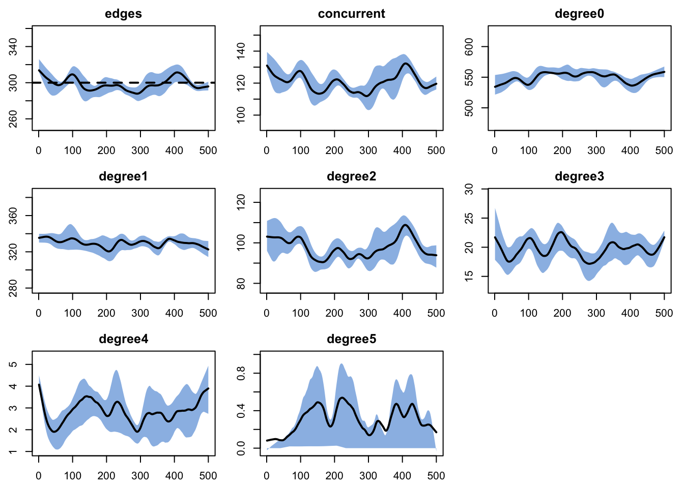
dx.mod2 <- netdx(est.mod2, nsims = nsims, ncores = ncores, nsteps = nsteps,
                 nwstats.formula = ~edges + concurrent + degree(0:5),
                 set.control.ergm = control.simulate.formula(MCMC.burnin = 1e5))
Network Diagnostics
-----------------------
- Simulating 5 networks
- Calculating formation statisticsprint(dx.mod2)EpiModel Network Diagnostics
=======================
Diagnostic Method: Dynamic
Simulations: 5
Time Steps per Sim: 500
Formation Diagnostics
-----------------------
Target Sim Mean Pct Diff Sim SE Z Score SD(Sim Means) SD(Statistic)
edges 300 295.057 -1.648 0.876 -5.646 1.630 8.948
concurrent 0 0.000 NaN NaN NaN 0.000 0.000
degree0 NA 409.886 NA 1.751 NA 3.259 17.895
degree1 NA 590.114 NA 1.751 NA 3.259 17.895
degree2 NA 0.000 NA NaN NA 0.000 0.000
degree3 NA 0.000 NA NaN NA 0.000 0.000
degree4 NA 0.000 NA NaN NA 0.000 0.000
degree5 NA 0.000 NA NaN NA 0.000 0.000
Duration Diagnostics
-----------------------
Target Sim Mean Pct Diff Sim SE Z Score SD(Sim Means) SD(Statistic)
edges 50 49.457 -1.086 0.336 -1.616 1.436 2.512
Dissolution Diagnostics
-----------------------
Target Sim Mean Pct Diff Sim SE Z Score SD(Sim Means) SD(Statistic)
edges 0.02 0.02 1.081 0 1.293 0 0.008plot(dx.mod2, plots.joined = FALSE)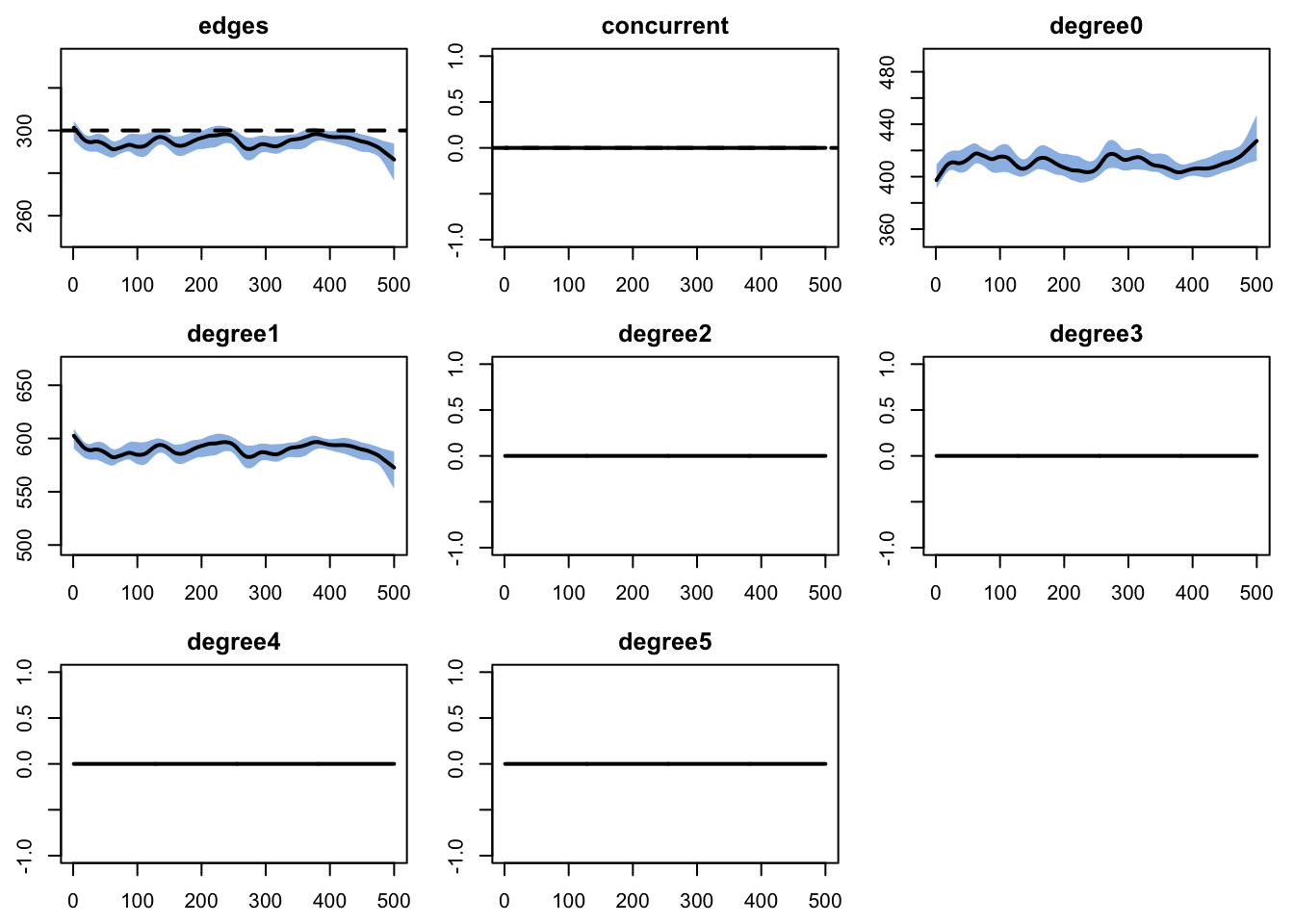
Epidemic Simulation
Epidemic Parameters
The two strains embody a classic trade-off: strain 1 is fast-and-furious (high per-act probability, short duration) while strain 2 is slow-and-steady (low per-act probability, long duration). The act.rate of 2 acts per partnership per week and the 50/50 initial strain split (pct.st2 = 0.5) are shared across both network scenarios.
param <- param.net(
1  inf.prob = 0.5, inf.prob.st2 = 0.01,
2  rec.rate = 0.05, rec.rate.st2 = 0.005,
  pct.st2 = 0.5,
  act.rate = 2
)

3init <- init.net(i.num = 50)

control <- control.net(
  type = NULL,
  nsims = nsims,
  ncores = ncores,
  nsteps = nsteps,
  initStrain.FUN = init_strain,
  recovery.FUN = recov.2strains,
  infection.FUN = infection.2strains,
  verbose = FALSE
)- 1
- Strain 1 transmits at 50% per act; strain 2 at 1% per act — a 50-fold difference in infectiousness.
- 2
- Strain 1 recovers in ~20 weeks on average; strain 2 in ~200 weeks — a 10-fold difference in duration.
- 3
-
50 initially infected nodes (5% prevalence), split evenly between strains by the
init_strainmodule.
Scenario 1: Concurrency Allowed
With concurrency, infected individuals can have multiple simultaneous partners. The acute strain (strain 1) exploits branching transmission chains — it can spread to a new partner before the existing partnership ends, even with a short infectious period.
sim.mod1 <- netsim(est.mod1, param, init, control)
print(sim.mod1)
EpiModel Simulation
=======================
Model class: netsim
Simulation Summary
-----------------------
Model type:
No. simulations: 5
No. time steps: 500
No. NW groups: 1
Fixed Parameters
---------------------------
inf.prob = 0.5
act.rate = 2
rec.rate = 0.05
inf.prob.st2 = 0.01
rec.rate.st2 = 0.005
pct.st2 = 0.5
groups = 1
Model Functions
-----------------------
initialize.FUN
resim_nets.FUN
summary_nets.FUN
infection.FUN
recovery.FUN
nwupdate.FUN
prevalence.FUN
verbose.FUN
initStrain.FUN
Model Output
-----------------------
Variables: s.num i.num num si.flow si.flow.st2 i.num.st1
i.num.st2 is.flow is.flow.st1 is.flow.st2
Networks: sim1 ... sim5
Transmissions: sim1 ... sim5
Formation Statistics
-----------------------
Target Sim Mean Pct Diff Sim SE Z Score SD(Sim Means) SD(Statistic)
edges 300 302.467 0.822 2.587 0.954 6.613 16.314
Duration Statistics
-----------------------
Target Sim Mean Pct Diff Sim SE Z Score SD(Sim Means) SD(Statistic)
edges 50 49.856 -0.289 0.401 -0.36 0.461 2.496
Dissolution Statistics
-----------------------
Target Sim Mean Pct Diff Sim SE Z Score SD(Sim Means) SD(Statistic)
edges 0.02 0.02 -0.428 0 -0.543 0 0.008Scenario 2: Strict Monogamy
Without concurrency, partnerships are sequential. Each new contact requires waiting for the current partnership to dissolve. The chronic strain (strain 2) persists across multiple sequential partnerships, giving it the advantage.
sim.mod2 <- netsim(est.mod2, param, init, control)
print(sim.mod2)
EpiModel Simulation
=======================
Model class: netsim
Simulation Summary
-----------------------
Model type:
No. simulations: 5
No. time steps: 500
No. NW groups: 1
Fixed Parameters
---------------------------
inf.prob = 0.5
act.rate = 2
rec.rate = 0.05
inf.prob.st2 = 0.01
rec.rate.st2 = 0.005
pct.st2 = 0.5
groups = 1
Model Functions
-----------------------
initialize.FUN
resim_nets.FUN
summary_nets.FUN
infection.FUN
recovery.FUN
nwupdate.FUN
prevalence.FUN
verbose.FUN
initStrain.FUN
Model Output
-----------------------
Variables: s.num i.num num si.flow si.flow.st2 i.num.st1
i.num.st2 is.flow is.flow.st1 is.flow.st2
Networks: sim1 ... sim5
Transmissions: sim1 ... sim5
Formation Statistics
-----------------------
Target Sim Mean Pct Diff Sim SE Z Score SD(Sim Means) SD(Statistic)
edges 300 297.283 -0.906 0.751 -3.616 1.054 8.429
concurrent 0 0.000 NaN NaN NaN 0.000 0.000
Duration Statistics
-----------------------
Target Sim Mean Pct Diff Sim SE Z Score SD(Sim Means) SD(Statistic)
edges 50 50.29 0.58 0.371 0.782 0.824 2.467
Dissolution Statistics
-----------------------
Target Sim Mean Pct Diff Sim SE Z Score SD(Sim Means) SD(Statistic)
edges 0.02 0.02 -0.138 0 -0.171 0 0.008Analysis
sim.mod1 <- mutate_epi(sim.mod1, prev = i.num / num,
                       prev.st1 = i.num.st1 / num,
                       prev.st2 = i.num.st2 / num)
sim.mod2 <- mutate_epi(sim.mod2, prev = i.num / num,
                       prev.st1 = i.num.st1 / num,
                       prev.st2 = i.num.st2 / num)
Strain Competition: Concurrency vs. Monogamy
The headline result: concurrency reverses which strain dominates. With concurrency, the fast-spreading strain 1 (red) dominates and may drive strain 2 to extinction. Under monogamy, the slow-and-steady strain 2 (blue) wins and strain 1 goes extinct.
par(mfrow = c(1, 2), mar = c(3, 3, 2, 1), mgp = c(2, 1, 0))
plot(sim.mod1, y = c("i.num.st1", "i.num.st2"),
     main = "Concurrency Allowed",
     ylab = "Infected (count)", xlab = "Week",
     mean.col = c("firebrick", "steelblue"), mean.lwd = 2, mean.smooth = TRUE,
     qnts.col = c("firebrick", "steelblue"), qnts.alpha = 0.2,
     qnts.smooth = TRUE, legend = TRUE)
plot(sim.mod2, y = c("i.num.st1", "i.num.st2"),
     main = "Strict Monogamy",
     ylab = "Infected (count)", xlab = "Week",
     mean.col = c("firebrick", "steelblue"), mean.lwd = 2, mean.smooth = TRUE,
     qnts.col = c("firebrick", "steelblue"), qnts.alpha = 0.2,
     qnts.smooth = TRUE, legend = TRUE)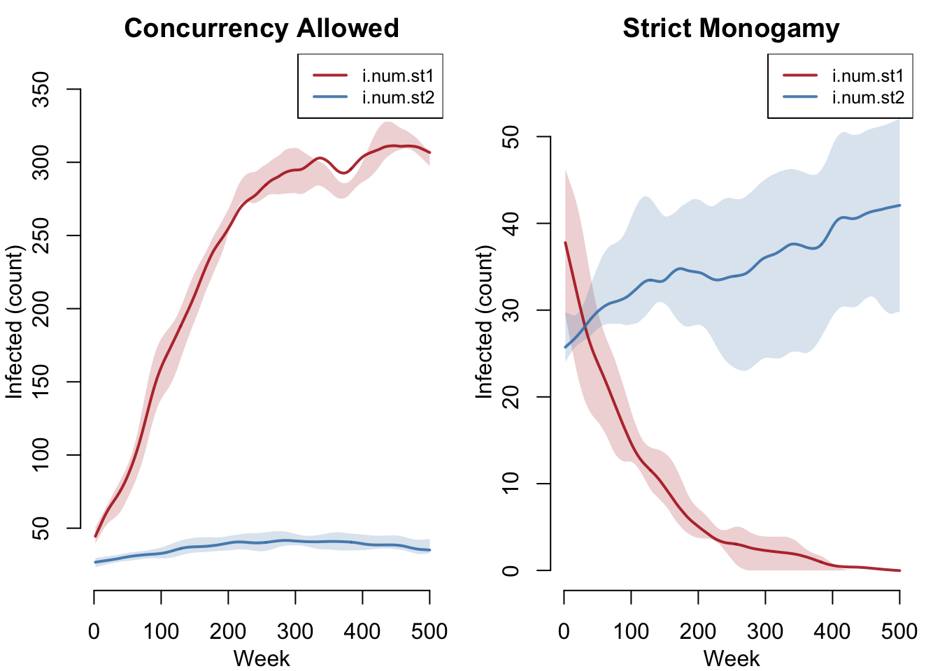
Total Prevalence Comparison
How does total disease burden compare across network structures? Both network models produce endemic disease, but the strain composition and overall prevalence differ.
par(mfrow = c(1, 1), mar = c(3, 3, 2, 1), mgp = c(2, 1, 0))
plot(sim.mod1, y = "prev",
     main = "Total Prevalence by Network Structure",
     ylab = "Prevalence (I / N)", xlab = "Week",
     mean.col = "firebrick", mean.lwd = 2, mean.smooth = TRUE,
     qnts.col = "firebrick", qnts.alpha = 0.2, qnts.smooth = TRUE,
     legend = FALSE)
plot(sim.mod2, y = "prev",
     mean.col = "steelblue", mean.lwd = 2, mean.smooth = TRUE,
     qnts.col = "steelblue", qnts.alpha = 0.2, qnts.smooth = TRUE,
     legend = FALSE, add = TRUE)
legend("topright",
       legend = c("Concurrency Allowed", "Strict Monogamy"),
       col = c("firebrick", "steelblue"), lwd = 2, bty = "n")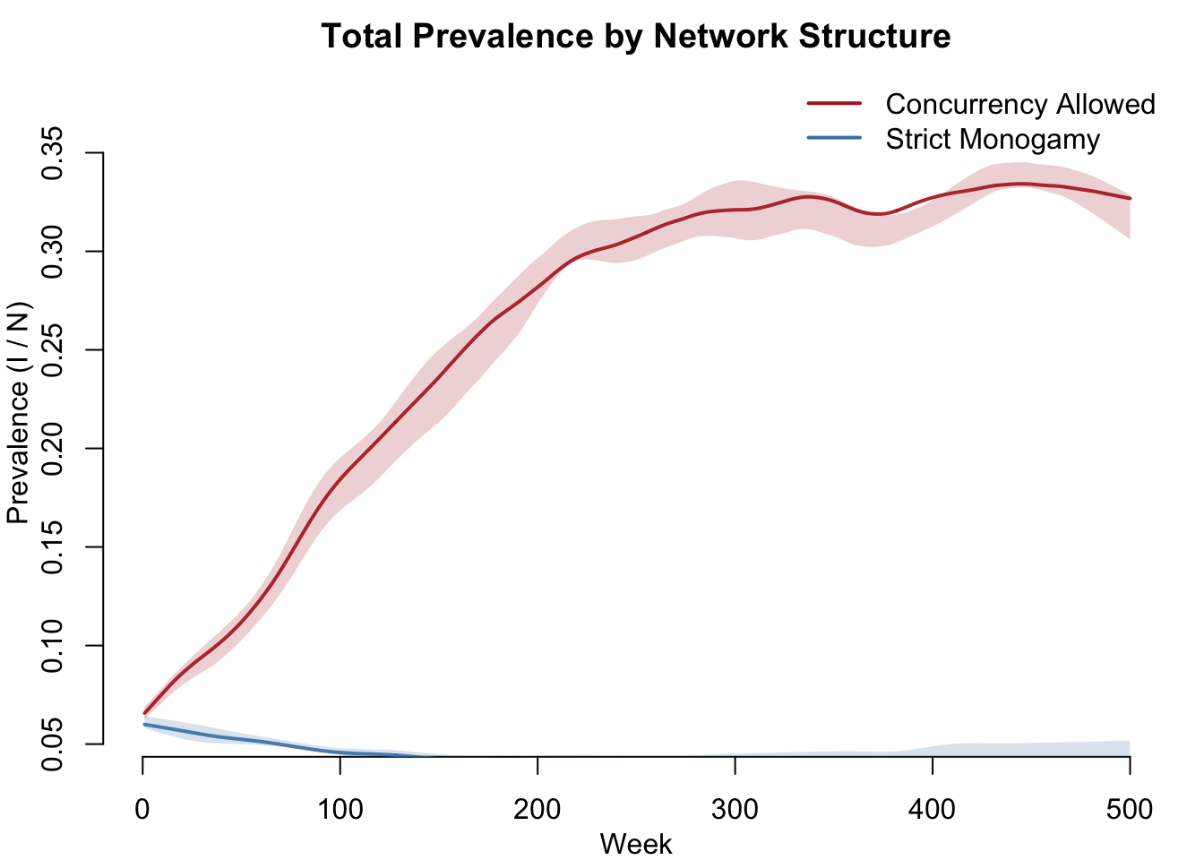
Incidence by Strain
New infections per week, broken out by strain and network model. This shows the transmission velocity of each strain under each network structure.
par(mfrow = c(1, 2), mar = c(3, 3, 2, 1), mgp = c(2, 1, 0))
plot(sim.mod1, y = c("si.flow", "si.flow.st2"),
     main = "Incidence: Concurrency",
     ylab = "New Infections / Week", xlab = "Week",
     mean.col = c("firebrick", "steelblue"),
     mean.lwd = 2, mean.smooth = TRUE,
     qnts = FALSE, legend = TRUE)
plot(sim.mod2, y = c("si.flow", "si.flow.st2"),
     main = "Incidence: Monogamy",
     ylab = "New Infections / Week", xlab = "Week",
     mean.col = c("firebrick", "steelblue"),
     mean.lwd = 2, mean.smooth = TRUE,
     qnts = FALSE, legend = TRUE)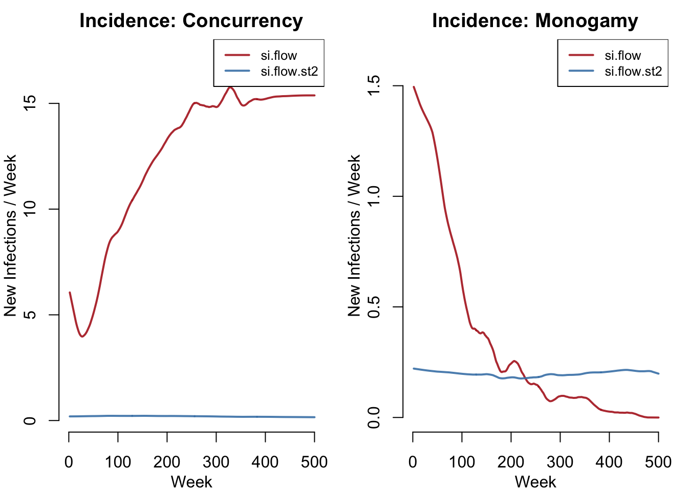
Summary Table
df1 <- as.data.frame(sim.mod1)
df2 <- as.data.frame(sim.mod2)

# Use last 20% of timesteps to estimate equilibrium
late1 <- df1$time > nsteps * 0.8
late2 <- df2$time > nsteps * 0.8

knitr::kable(data.frame(
  Metric = c("Equilibrium prevalence (total)",
             "Strain 1 prevalence",
             "Strain 2 prevalence",
             "Dominant strain",
             "Cumulative infections (St1)",
             "Cumulative infections (St2)"),
  Concurrency = c(
    round(mean(df1$prev[late1], na.rm = TRUE), 3),
    round(mean(df1$prev.st1[late1], na.rm = TRUE), 3),
    round(mean(df1$prev.st2[late1], na.rm = TRUE), 3),
    ifelse(mean(df1$i.num.st1[late1], na.rm = TRUE) >
             mean(df1$i.num.st2[late1], na.rm = TRUE),
           "Strain 1", "Strain 2"),
    round(mean(tapply(df1$si.flow, df1$sim, sum, na.rm = TRUE))),
    round(mean(tapply(df1$si.flow.st2, df1$sim, sum, na.rm = TRUE)))
  ),
  Monogamy = c(
    round(mean(df2$prev[late2], na.rm = TRUE), 3),
    round(mean(df2$prev.st1[late2], na.rm = TRUE), 3),
    round(mean(df2$prev.st2[late2], na.rm = TRUE), 3),
    ifelse(mean(df2$i.num.st1[late2], na.rm = TRUE) >
             mean(df2$i.num.st2[late2], na.rm = TRUE),
           "Strain 1", "Strain 2"),
    round(mean(tapply(df2$si.flow, df2$sim, sum, na.rm = TRUE))),
    round(mean(tapply(df2$si.flow.st2, df2$sim, sum, na.rm = TRUE)))
  )
))| Metric | Concurrency | Monogamy |
|---|---|---|
| Equilibrium prevalence (total) | 0.34 | 0.032 |
| Strain 1 prevalence | 0.331 | 0 |
| Strain 2 prevalence | 0.026 | 0.032 |
| Dominant strain | Strain 1 | Strain 2 |
| Cumulative infections (St1) | 6402 | 145 |
| Cumulative infections (St2) | 72 | 85 |
Sensitivity Analysis: Concurrency Gradient
TipTry It Yourself
The code below sweeps across 13 concurrency levels, re-estimating the network and running the epidemic at each level. This takes several minutes to run. The code is shown for reference — copy it into an interactive R session to explore the results.
formation.mod3 <- ~edges + concurrent
concties.mod3 <- seq(0, 120, 10)
est.mod3 <- list()
sim.mod3 <- list()

for (i in seq_along(concties.mod3)) {
  target.stats.mod3 <- c(300, concties.mod3[i])
  est.mod3[[i]] <- suppressMessages(
    netest(nw, formation.mod3, target.stats.mod3, coef.diss)
  )
  sim.mod3[[i]] <- netsim(est.mod3[[i]], param, init, control)
}

# Extract equilibrium strain prevalence (last timestep mean)
i.num.st1.final <- sapply(seq_along(concties.mod3), function(x) {
  tail(as.data.frame(sim.mod3[[x]], out = "mean")[["i.num.st1"]], 1)
})
i.num.st2.final <- sapply(seq_along(concties.mod3), function(x) {
  tail(as.data.frame(sim.mod3[[x]], out = "mean")[["i.num.st2"]], 1)
})

# Plot the gradient
par(mfrow = c(1, 1), mar = c(3, 3, 2, 1), mgp = c(2, 1, 0))
plot(concties.mod3, i.num.st1.final, type = "b", pch = 19,
     col = "firebrick", lwd = 2,
     xlab = "Nodes with Concurrent Ties",
     ylab = "Equilibrium Infected (count)",
     main = "Strain Competition vs. Concurrency",
     ylim = c(0, max(c(i.num.st1.final, i.num.st2.final), na.rm = TRUE)))
points(concties.mod3, i.num.st2.final, type = "b", pch = 19,
       col = "steelblue", lwd = 2)
legend("topleft",
       legend = c("Strain 1 (acute)", "Strain 2 (chronic)"),
       col = c("firebrick", "steelblue"), lwd = 2, pch = 19, bty = "n")
Parameters
Transmission
| Parameter | Description | Default |
|---|---|---|
inf.prob |
Per-act transmission probability (strain 1) | 0.5 |
inf.prob.st2 |
Per-act transmission probability (strain 2) | 0.01 |
act.rate |
Acts per partnership per week | 2 |
Recovery
| Parameter | Description | Default |
|---|---|---|
rec.rate |
Recovery rate, strain 1 (mean ~20 weeks) | 0.05 |
rec.rate.st2 |
Recovery rate, strain 2 (mean ~200 weeks) | 0.005 |
Strain Initialization
| Parameter | Description | Default |
|---|---|---|
pct.st2 |
Probability initial infection is strain 2 | 0.5 |
Optional Intervention
| Parameter | Description | Default |
|---|---|---|
inter.eff |
Intervention efficacy (reduces transmission by this factor) | Not set |
inter.start |
Timestep when intervention begins | Not set |
Network
| Parameter | Description | Default |
|---|---|---|
| Population size | Number of nodes | 1000 |
| Target edges | Mean concurrent partnerships | 300 |
| Concurrency | Varies by model (0 or ~120) | — |
| Partnership duration | Mean edge duration (weeks) | 50 |
Module Execution Order
resim_nets → initStrain → infection → recovery → prevalenceThe initStrain module runs first (but only operates at the first timestep). Infection runs before recovery so that newly infected individuals can be tracked before any recovery occurs in the same timestep.
Next Steps
- Add co-infection: Allow individuals to carry both strains simultaneously, introducing within-host competition and superinfection dynamics
- Model strain mutation: Allow strain 1 to mutate into strain 2 (or vice versa), exploring the evolution of virulence
- Add vital dynamics: Introduce births and deaths to study longer-term strain competition — see SI with Vital Dynamics
- Vary the trade-off: Explore different points on the infectiousness-duration trade-off curve to map the full parameter space of competitive outcomes
- Add a treatment intervention: Differential treatment efficacy across strains connects to antimicrobial resistance — see Test and Treat
- Extend to three or more strains: Generalize the framework to model multi-strain competition with more complex fitness landscapes