Epidemics over Observed Networks

observed networks

census data

intermediate

SI epidemic simulation over observed (census) dynamic networks without ERGM estimation

Author

Samuel M. Jenness

Published

August 1, 2018

Overview

The standard EpiModel workflow begins with egocentrically observed network data, fits a temporal ERGM (exponential random graph model) with the generative network effects of interest, and then simulates from that model fit over time. This example demonstrates an alternative approach: using a dynamic network census where all nodes and edges are directly observed over a series of discrete time steps. Rather than fitting and simulating from a statistical network model, the observed networkDynamic object is placed directly into the simulation data structure.

This is the only gallery example that bypasses EpiModel’s ERGM estimation and simulation pipeline entirely. The resimulate.network parameter is set to FALSE so the network is used as-is rather than being regenerated at each timestep. Because there is no model fit, this approach requires custom initialization and infection modules that handle the observed network directly.

Two scenarios are demonstrated using a simulated dataset from the networkDynamicData package (treated as if it were an observed network census): a basic SI model with constant transmission probability, and a two-stage disease model with time-varying transmission probability and network visualization. An important caveat — the observed network has edge activity recorded over a finite window, so nsteps must match the number of observed time steps — is also explored.

Source Files

Download the individual source files for this example:

model.R — Main simulation script
module-fx.R — Custom module functions

Model Structure

Compartments

Compartment	Label	Description
Susceptible	S	Not infected; at risk of infection through network contacts
Infectious	I	Infected; can transmit to susceptible partners

Flow Diagram

flowchart LR
    S["<b>S</b><br/>Susceptible"] -->|"infection<br/>(si.flow)"| I["<b>I</b><br/>Infectious"]

    style S fill:#3498db,color:#fff
    style I fill:#e74c3c,color:#fff

This is a simple SI model with no recovery. In a closed population without vital dynamics, prevalence increases monotonically toward saturation.

Observed Network Data

Unlike other gallery examples, this model does not call netest() to fit an ERGM. Instead, the observed networkDynamic object contains edge spells (onset/terminus times for each partnership) recorded over approximately 100 discrete time steps. Key characteristics of the network:

1000 nodes in an undirected network
Edge spells define when each partnership is active
The existing status.active vertex attribute is removed before simulation, since we simulate our own epidemic
No network resimulation — the observed edge structure is fixed throughout the simulation

Setup

library(EpiModel)
library(networkDynamicData)

Simulation Parameters

nsims <- 5
ncores <- 5
nsteps <- 100

Custom Modules

This example requires two custom modules because the standard EpiModel initialization and infection modules expect a netest object (a fitted ERGM). Since we are working with an observed network that has no model fit, we need custom functions that handle the network directly.

Initialization Module

The init_obsnw function replaces EpiModel’s built-in initialize.net. It creates the master data list, places the observed networkDynamic object directly into the simulation data structure, initializes node attributes, and randomly assigns initial infections. When track.nw.attr = TRUE, it also stores time-varying disease status on the network as a temporally extended attribute (TEA), enabling network visualization with color-coded disease status.

init_obsnw <- function(x, param, init, control, s) {

1  dat <- create_dat_object(param, init, control)

  dat$num.nw <- 1L
2  dat$run$nw[[1]] <- x
  dat <- set_param(dat, "groups", 1)

  i.num <- get_init(dat, "i.num")
  n <- network.size(dat$run$nw[[1]])
  dat <- append_core_attr(dat, 1, n)

  status <- rep("s", n)
3  status[sample(1:n, i.num)] <- "i"
  dat <- set_attr(dat, "status", status)

  infTime <- rep(NA, n)
  infTime[which(status == "i")] <- 1
  dat <- set_attr(dat, "infTime", infTime)

  track.nw.attr <- get_param(dat, "track.nw.attr",
                              override.null.error = TRUE)
  if (!is.null(track.nw.attr) && track.nw.attr) {
4    dat$run$nw[[1]] <- networkDynamic::activate.vertex.attribute(
      dat$run$nw[[1]], prefix = "testatus",
      value = get_attr(dat, "status"), onset = 1, terminus = Inf
    )
  }

5  dat <- prevalence.net(dat, 1)
  return(dat)
}

1: Create the master data list from parameters, initial conditions, and control settings.
2: Place the observed networkDynamic object directly into the data structure — no ERGM fit needed.
3: Randomly assign i.num initial infections among the n network nodes.
4: When track.nw.attr = TRUE, store disease status as a temporally extended attribute on the network for visualization.
5: Call the built-in prevalence.net() to record initial epidemic statistics.

Infection Module

The infect_obsnw function handles transmission over the observed network. It supports two modes selected automatically based on which parameters are provided: a simple mode with constant transmission probability (inf.prob) and a time-varying mode where transmission depends on infection duration (inf.prob.stage1 / inf.prob.stage2).

infect_obsnw <- function(dat, at) {

  active <- get_attr(dat, "active")
  status <- get_attr(dat, "status")
  infTime <- get_attr(dat, "infTime")

  act.rate <- get_param(dat, "act.rate")
  inf.prob.stage1 <- get_param(dat, "inf.prob.stage1",
                                override.null.error = TRUE)

1  time_varying <- !is.null(inf.prob.stage1)
  if (time_varying) {
    inf.prob.stage2 <- get_param(dat, "inf.prob.stage2")
    dur.stage1 <- get_param(dat, "dur.stage1")
  } else {
    inf.prob <- get_param(dat, "inf.prob")
  }

  idsInf <- which(active == 1 & status == "i")
  nActive <- sum(active == 1)
  nElig <- length(idsInf)

  totInf <- 0

  if (nElig > 0 && nElig < nActive) {

2    del <- discord_edgelist(dat, at)

    if (!is.null(del)) {

      if (time_varying) {
        infDur.del <- at - infTime[del$inf]
3        del$transProb <- ifelse(infDur.del <= dur.stage1,
                                inf.prob.stage1, inf.prob.stage2)
      } else {
        del$transProb <- inf.prob
      }

      del$actRate <- act.rate
      del$finalProb <- 1 - (1 - del$transProb) ^ del$actRate
      transmit <- rbinom(nrow(del), 1, del$finalProb)
      del <- del[which(transmit == 1), ]

      idsNewInf <- unique(del$sus)
      totInf <- length(idsNewInf)

      if (totInf > 0) {
        status[idsNewInf] <- "i"
        infTime[idsNewInf] <- at
        dat <- set_attr(dat, "status", status)
        dat <- set_attr(dat, "infTime", infTime)

        track.nw.attr <- get_param(dat, "track.nw.attr",
                                   override.null.error = TRUE)
        if (!is.null(track.nw.attr) && track.nw.attr) {
          dat$run$nw[[1]] <-
4            networkDynamic::activate.vertex.attribute(
              dat$run$nw[[1]], prefix = "testatus",
              value = "i", onset = at, terminus = Inf, v = idsNewInf
            )
        }
      }
    }
  }

5  dat <- set_epi(dat, "si.flow", at, totInf)

  return(dat)
}

1: Automatically detect whether to use time-varying transmission based on whether inf.prob.stage1 was specified in the parameters.
2: Use discord_edgelist() to identify susceptible–infectious partnerships active at the current timestep.
3: In time-varying mode, assign transmission probability based on how long each infector has been infected relative to dur.stage1.
4: Update the temporally extended attribute on the network so newly infected nodes are visualized correctly.
5: Record the number of new infections at this timestep as the si.flow epidemic tracker.

Network Model

Loading the Observed Network

The concurrencyComparisonNets dataset from the networkDynamicData package provides an observed dynamic network. We extract the base network and remove the existing disease status attribute, since we will simulate our own epidemic.

data(concurrencyComparisonNets)
nw <- base
print(nw)

NetworkDynamic properties:
  distinct change times: 104 
  maximal time range: -Inf until  Inf 

 Dynamic (TEA) attributes:
  Vertex TEAs:    status.active 

Includes optional net.obs.period attribute:
 Network observation period info:
  Number of observation spells: 1 
  Maximal time range observed: 2 until 102 
  Temporal mode: discrete 
  Time unit: step 
  Suggested time increment: 1 

 Network attributes:
  vertices = 1000 
  directed = FALSE 
  hyper = FALSE 
  loops = FALSE 
  multiple = FALSE 
  bipartite = FALSE 
  net.obs.period: (not shown)
  total edges= 1916 
    missing edges= 0 
    non-missing edges= 1916 

 Vertex attribute names: 
    status.active vertex.names 

 Edge attribute names not shown

nw <- network::delete.vertex.attribute(nw, "status.active")

Epidemic Simulation

Example 1: Basic SI Epidemic

The first scenario uses a simple SI model with a constant per-act transmission probability of 50% and a single act per partnership per timestep.

param <- param.net(inf.prob = 0.5, act.rate = 1)
init <- init.net(i.num = 10)

The control settings specify our custom modules and disable network resimulation and network statistics saving (since there is no ERGM fit to compute statistics from). The nsteps parameter is set to match the number of observed time steps in the network.

control <- control.net(
  type = NULL,
  nsteps = nsteps,
  nsims = nsims,
  ncores = ncores,
  initialize.FUN = init_obsnw,
  infection.FUN = infect_obsnw,
  prevalence.FUN = prevalence.net,
  resimulate.network = FALSE,
  save.nwstats = FALSE,
  verbose = FALSE
)

sim <- netsim(nw, param, init, control)
print(sim)

EpiModel Simulation
=======================
Model class: netsim

Simulation Summary
-----------------------
Model type:
No. simulations: 5
No. time steps: 100
No. NW groups: 1

Fixed Parameters
---------------------------
inf.prob = 0.5
act.rate = 1
groups = 1

Model Functions
-----------------------
initialize.FUN 
resim_nets.FUN 
summary_nets.FUN 
infection.FUN 
nwupdate.FUN 
prevalence.FUN 
verbose.FUN 

Model Output
-----------------------
Variables: s.num i.num num si.flow
Networks: sim1 ... sim5
Transmissions: sim1 ... sim5

df <- as.data.frame(sim)
head(df, 25)

   sim time s.num i.num  num si.flow
1    1    1   990    10 1000      NA
2    1    2   988    12 1000       2
3    1    3   987    13 1000       1
4    1    4   983    17 1000       4
5    1    5   981    19 1000       2
6    1    6   976    24 1000       5
7    1    7   975    25 1000       1
8    1    8   973    27 1000       2
9    1    9   970    30 1000       3
10   1   10   966    34 1000       4
11   1   11   961    39 1000       5
12   1   12   956    44 1000       5
13   1   13   954    46 1000       2
14   1   14   952    48 1000       2
15   1   15   949    51 1000       3
16   1   16   946    54 1000       3
17   1   17   943    57 1000       3
18   1   18   940    60 1000       3
19   1   19   938    62 1000       2
20   1   20   934    66 1000       4
21   1   21   928    72 1000       6
22   1   22   924    76 1000       4
23   1   23   921    79 1000       3
24   1   24   920    80 1000       1
25   1   25   915    85 1000       5

Caveats: Simulating Past the Observation Window

The observed network has edge activity recorded over a finite window of approximately 100 timesteps. Edges that are active at the last observed time remain active indefinitely (a networkDynamic convention). This means nothing prevents simulating past the observation window — but the results become meaningless: the frozen edge set no longer reflects real dynamics, prevalence plateaus, and incidence drops to zero.

head(get.dyads.active(nw, at = 1), 10)

      [,1] [,2]
 [1,]  834    4
 [2,]  251    9
 [3,]  722    9
 [4,]   93   10
 [5,]  169   10
 [6,]   37   12
 [7,]  309   13
 [8,]  295   23
 [9,]  187   26
[10,]  564   27

head(get.dyads.active(nw, at = 100), 10)

      [,1] [,2]
 [1,]  445   46
 [2,]  464   78
 [3,]  380  270
 [4,]  777  365
 [5,]  850  808
 [6,]   14  852
 [7,]  308  868
 [8,]  664  711
 [9,]  428  930
[10,]  534  780

head(get.dyads.active(nw, at = 200), 10)

      [,1] [,2]
 [1,]  445   46
 [2,]  464   78
 [3,]  380  270
 [4,]  777  365
 [5,]  850  808
 [6,]   14  852
 [7,]  664  711
 [8,]  428  930
 [9,]  534  780
[10,]   50  242

To demonstrate this problem, we simulate 200 timesteps on the approximately 100-step network:

control_caveat <- control.net(
  type = NULL,
  nsteps = 200,
  nsims = nsims,
  ncores = ncores,
  initialize.FUN = init_obsnw,
  infection.FUN = infect_obsnw,
  prevalence.FUN = prevalence.net,
  resimulate.network = FALSE,
  save.nwstats = FALSE,
  verbose = FALSE
)

sim_caveat <- netsim(nw, param, init, control_caveat)

par(mfrow = c(1, 2), mar = c(3, 3, 2, 1), mgp = c(2, 1, 0))
plot(sim_caveat, y = "i.num",
     main = "Prevalence (Past Observations)",
     ylab = "Infected Count", xlab = "Time Step",
     mean.col = "firebrick", mean.lwd = 2, mean.smooth = FALSE,
     qnts.col = "firebrick", qnts.alpha = 0.2, qnts.smooth = FALSE,
     legend = FALSE)
plot(sim_caveat, y = "si.flow",
     main = "Incidence (Past Observations)",
     ylab = "New Infections", xlab = "Time Step",
     mean.col = "steelblue", mean.lwd = 2, mean.smooth = FALSE,
     qnts.col = "steelblue", qnts.alpha = 0.2, qnts.smooth = FALSE,
     legend = FALSE)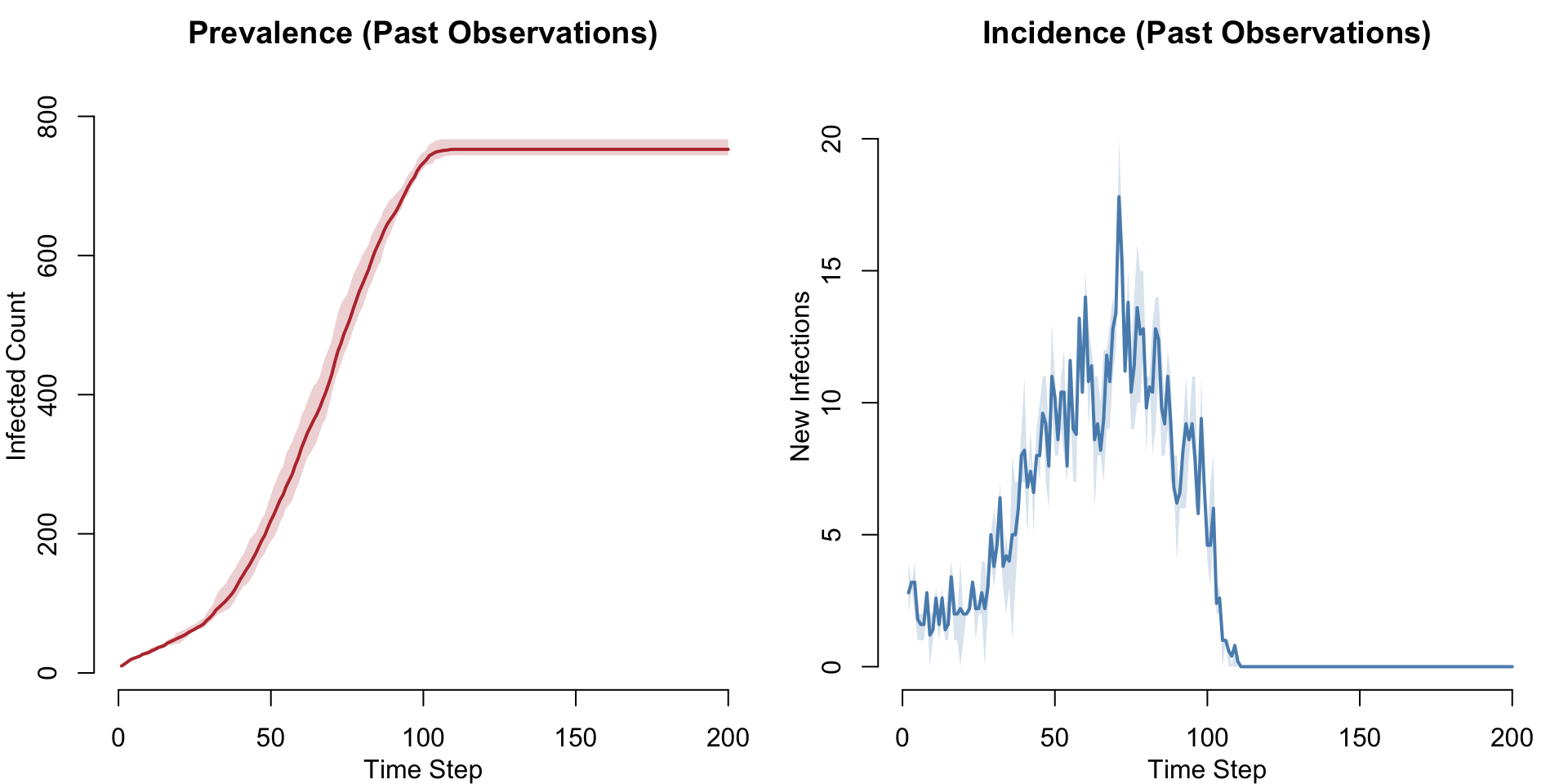

Figure 1: Simulating past the observation window causes prevalence to plateau and incidence to drop to zero as the frozen edge set no longer reflects real network dynamics.

The takeaway: always match nsteps to the number of observed time steps in the network.

Example 2: Time-Varying Transmission

The second scenario models a two-stage disease where transmission probability depends on infection duration. During the primary stage (first 5 timesteps after infection), transmission probability is low (5% per act); during the secondary stage, it increases (15% per act). The track.nw.attr = TRUE parameter stores time-varying disease status on the network, enabling network visualization.

param <- param.net(
  inf.prob.stage1 = 0.05,
  inf.prob.stage2 = 0.15,
  dur.stage1 = 5,
  act.rate = 1,
  track.nw.attr = TRUE
)
init <- init.net(i.num = 10)

control <- control.net(
  type = NULL,
  nsteps = nsteps,
  nsims = nsims,
  ncores = ncores,
  initialize.FUN = init_obsnw,
  infection.FUN = infect_obsnw,
  prevalence.FUN = prevalence.net,
  resimulate.network = FALSE,
  save.nwstats = FALSE,
  verbose = FALSE
)

sim2 <- netsim(nw, param, init, control)
print(sim2)

EpiModel Simulation
=======================
Model class: netsim

Simulation Summary
-----------------------
Model type:
No. simulations: 5
No. time steps: 100
No. NW groups: 1

Fixed Parameters
---------------------------
act.rate = 1
inf.prob.stage1 = 0.05
inf.prob.stage2 = 0.15
dur.stage1 = 5
track.nw.attr = TRUE
groups = 1

Model Functions
-----------------------
initialize.FUN 
resim_nets.FUN 
summary_nets.FUN 
infection.FUN 
nwupdate.FUN 
prevalence.FUN 
verbose.FUN 

Model Output
-----------------------
Variables: s.num i.num num si.flow
Networks: sim1 ... sim5
Transmissions: sim1 ... sim5

Network Visualization

Because track.nw.attr = TRUE, we can visualize the network colored by disease status at different time points.

par(mfrow = c(1, 2), mar = c(1, 1, 1, 1))
plot(sim2, type = "network", col.status = TRUE, at = 2, sims = 1)
plot(sim2, type = "network", col.status = TRUE, at = nsteps, sims = 1)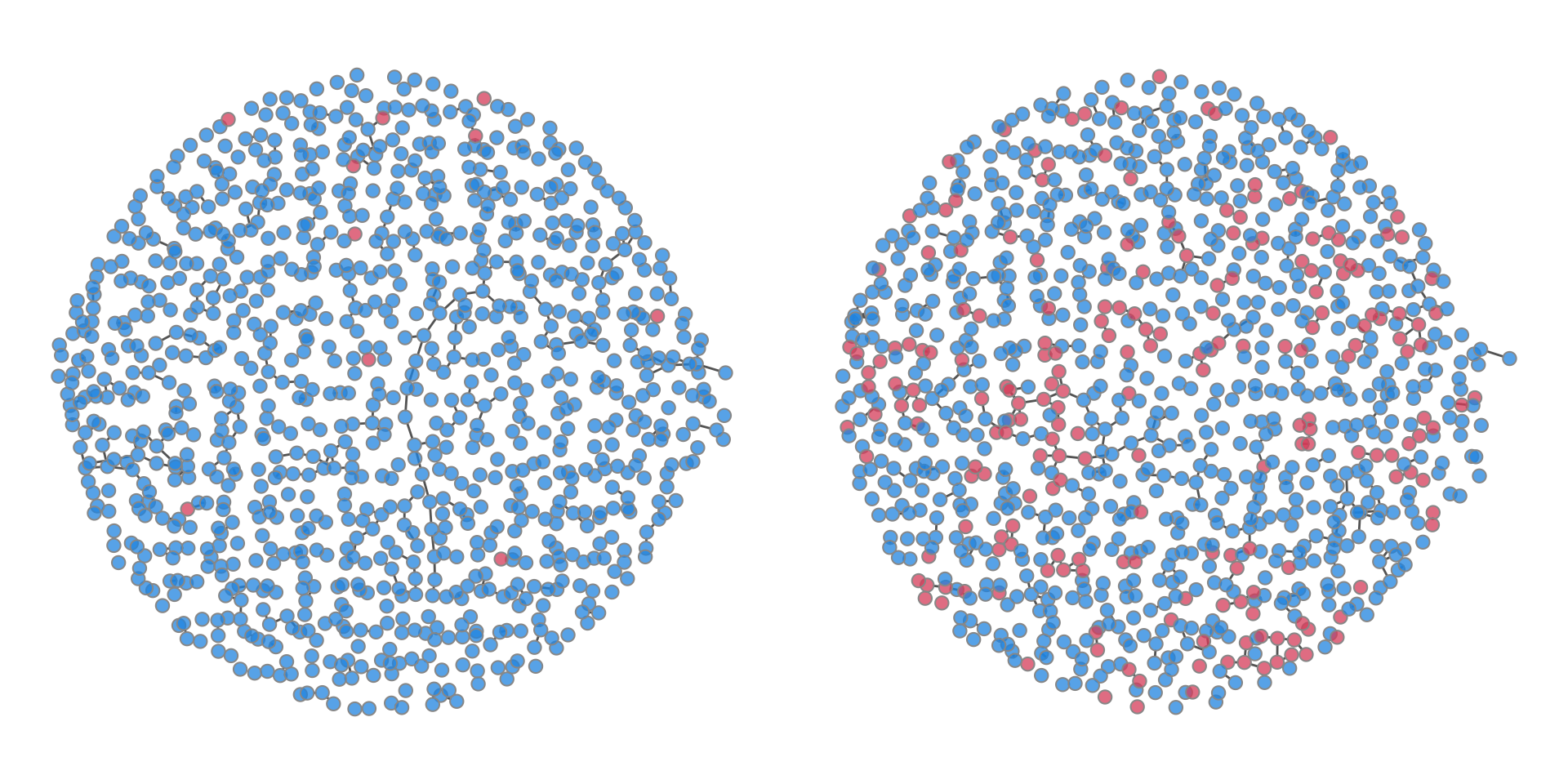

Figure 2: Network snapshots colored by disease status at early (left) and late (right) time steps. Blue nodes are susceptible; red nodes are infectious.

Extracting Individual-Level Data

The time-varying disease status stored on the network can be extracted at any time point using the networkDynamic API:

nwd <- get_network(sim2, 1)
head(get.vertex.attribute.active(nwd, "testatus", at = 1), 25)

 [1] "s" "s" "s" "s" "s" "s" "s" "i" "s" "s" "s" "s" "s" "s" "s" "s" "s" "s" "s"
[20] "s" "s" "s" "s" "s" "s"

head(get.vertex.attribute.active(nwd, "testatus", at = nsteps), 25)

 [1] "s" "s" "s" "s" "s" "s" "s" "i" "s" "s" "i" "i" "s" "s" "s" "s" "i" "s" "i"
[20] "i" "s" "i" "s" "s" "s"

Analysis

Prevalence Comparison

sim <- mutate_epi(sim, prev = i.num / num)
sim2 <- mutate_epi(sim2, prev = i.num / num)

par(mfrow = c(1, 2), mar = c(3, 3, 2, 1), mgp = c(2, 1, 0))
plot(sim, y = "i.num",
     main = "Ex 1: Constant Transmission",
     ylab = "Infected Count", xlab = "Time Step",
     mean.col = "firebrick", mean.lwd = 2, mean.smooth = TRUE,
     qnts.col = "firebrick", qnts.alpha = 0.2, qnts.smooth = TRUE,
     legend = FALSE)
plot(sim2, y = "i.num",
     main = "Ex 2: Time-Varying Transmission",
     ylab = "Infected Count", xlab = "Time Step",
     mean.col = "firebrick", mean.lwd = 2, mean.smooth = TRUE,
     qnts.col = "firebrick", qnts.alpha = 0.2, qnts.smooth = TRUE,
     legend = FALSE)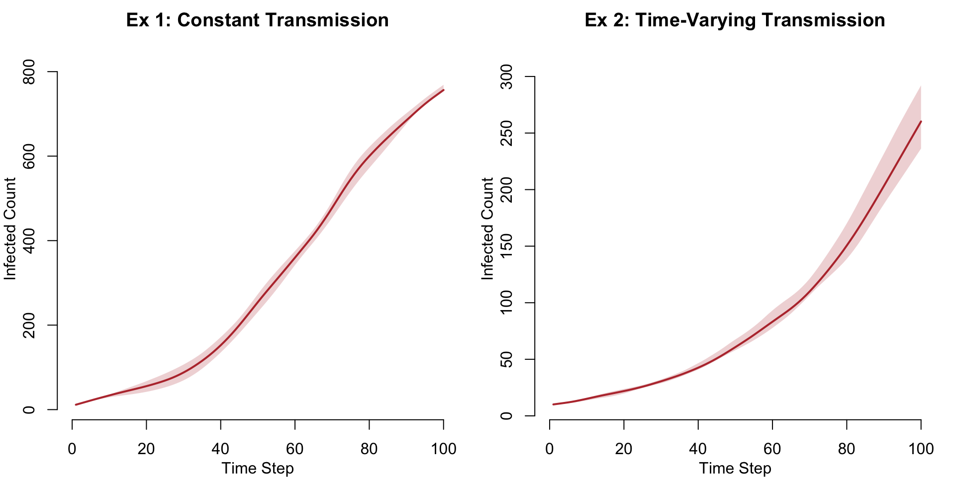

Figure 3: Prevalence over time for the constant transmission scenario (left) and the time-varying transmission scenario (right). The high constant transmission probability produces rapid saturation, while the lower time-varying probabilities yield a slower epidemic trajectory.

Incidence Comparison

par(mfrow = c(1, 2), mar = c(3, 3, 2, 1), mgp = c(2, 1, 0))
plot(sim, y = "si.flow",
     main = "Ex 1: Incidence",
     ylab = "New Infections", xlab = "Time Step",
     mean.col = "steelblue", mean.lwd = 2, mean.smooth = TRUE,
     qnts.col = "steelblue", qnts.alpha = 0.2, qnts.smooth = TRUE,
     legend = FALSE)
plot(sim2, y = "si.flow",
     main = "Ex 2: Incidence",
     ylab = "New Infections", xlab = "Time Step",
     mean.col = "steelblue", mean.lwd = 2, mean.smooth = TRUE,
     qnts.col = "steelblue", qnts.alpha = 0.2, qnts.smooth = TRUE,
     legend = FALSE)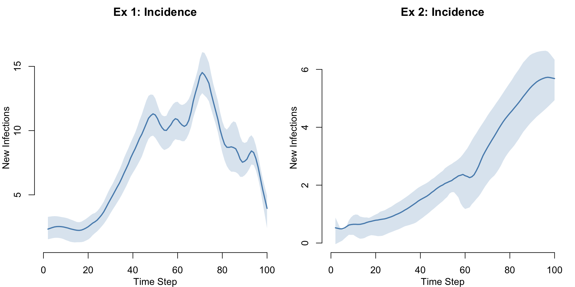

Figure 4: New infections per timestep for the constant transmission scenario (left) and the time-varying transmission scenario (right). High constant transmission produces a rapid initial surge that declines as susceptibles are depleted.

Summary Table

Table 1

df1 <- as.data.frame(sim)
df2 <- as.data.frame(sim2)

data.frame(
  Metric = c("Final prevalence",
             "Cumulative infections",
             "Mean incidence per step"),
  Example1 = c(
    round(mean(df1$prev[df1$time == max(df1$time)], na.rm = TRUE), 3),
    round(mean(tapply(df1$si.flow, df1$sim, sum, na.rm = TRUE))),
    round(mean(df1$si.flow, na.rm = TRUE), 2)
  ),
  Example2 = c(
    round(mean(df2$prev[df2$time == max(df2$time)], na.rm = TRUE), 3),
    round(mean(tapply(df2$si.flow, df2$sim, sum, na.rm = TRUE))),
    round(mean(df2$si.flow, na.rm = TRUE), 2)
  )
)

                   Metric Example1 Example2
1        Final prevalence    0.754     0.26
2   Cumulative infections  744.000   250.00
3 Mean incidence per step    7.510     2.53

Parameters

Example 1: Basic SI

Parameter	Description	Value
`inf.prob`	Per-act transmission probability	0.5
`act.rate`	Acts per partnership per timestep	1
`i.num`	Initial number of infected nodes	10

Example 2: Time-Varying Transmission

Parameter	Description	Value
`inf.prob.stage1`	Transmission probability during primary stage	0.05
`inf.prob.stage2`	Transmission probability during secondary stage	0.15
`dur.stage1`	Duration of primary stage (timesteps)	5
`act.rate`	Acts per partnership per timestep	1
`track.nw.attr`	Track time-varying disease status on network for visualization	TRUE
`i.num`	Initial number of infected nodes	10

Module Execution Order

At each timestep, modules execute in the following order:

Order	Module	Function	Description
1	Initialization	`init_obsnw`	Set up data structure, place observed network, assign initial infections (timestep 1 only)
2	Infection	`infect_obsnw`	Identify discordant partnerships, compute transmission, update infection status
3	Prevalence	`prevalence.net`	Record compartment sizes and flows (built-in EpiModel function)

Note that unlike most gallery examples, there is no network resimulation step. The resimulate.network = FALSE setting means the observed network is used as-is at every timestep, preserving the exact partnership structure from the census data.

Next Steps

Add recovery or immunity: Convert this to an SIS or SIR model by adding a recovery module — see the SEIR with Exposed State example for how additional compartments are implemented
Add vital dynamics: Introduce births and deaths to study longer-term epidemics — see SI with Vital Dynamics
Use a different dataset: The networkDynamicData package contains several other observed dynamic networks that could be substituted
Bridge approaches: Take a static network dataset (e.g., from the ergm package) and fit a TERGM with an assumed edge dissolution rate, combining observed and model-based methods