Partner Notification for an Endemic Bacterial STI

Partner notification for a chlamydia-like infection without immunity, in a heterosexual population of young adults with main and casual partnerships. A partner services module finds each diagnosed person’s recent partners through EpiModel’s cumulative edgelist and treats them by patient referral or expedited partner therapy. Every scenario resumes the same burn-in to endemic equilibrium, and the page reports prevalence, infections averted with Monte Carlo intervals, repeat infection of cured cases and its source, and whom partner services reaches.

Overview

Partner notification is the partner services intervention for sexually transmitted infections: when a person is diagnosed, the people they recently had sex with are told that they were exposed and are offered treatment. For a curable bacterial infection that leaves no immunity, such as chlamydia, it does two jobs. It finds infections in partners, most of which cause no symptoms and would otherwise go untested, and it protects the person who was just treated, because an untreated partner who is still infected will reinfect them (Heijne et al. 2011). The second job has no counterpart in contact tracing for an immunizing infection, and it is why the CDC treatment guidelines make partner treatment part of the clinical management of the index case rather than only a public health activity.

Both jobs run through a sexual network. The partners who matter are the partners the index case actually had over a lookback window, some of them in partnerships that have already ended, and whether a partner can be reached depends on the kind of partnership it was. EpiModel keeps the record that makes this computable, the cumulative edgelist: every partnership the simulation has seen, in every network layer, with the steps on which it began and ended. This example uses it to model partner services for a chlamydia-like infection among heterosexual young adults, and to ask four questions from the trials and models of partner notification:

1. What does partner notification contribute? The burn-in runs screening with patient referral (PR), in which the index case is asked to tell their partners, who then come in to be tested and treated. That is the usual standard of care in the United States, and the model is tuned to about 3% prevalence under it. Removing it shows what it contributes.
2. Patient referral or expedited partner therapy? Under expedited partner therapy (EPT) the index case delivers medication to their partners. Trials found that it gets more partners treated and reduces repeat infection of the index case by about a quarter for chlamydia and gonorrhea combined, with smaller reductions for chlamydia alone that did not reach statistical significance (Golden et al. 2005; Schillinger et al. 2003; Ferreira et al. 2013). It also gives something up: partners are never tested, so an infected partner is not diagnosed, and that partner’s own partners are never notified. Patient referral keeps that chain.
3. How far back? CDC guidance notifies partners from the 60 days before diagnosis; UK guidance uses six months for most cases (McClean et al. 2013). A third option gives EPT to ongoing partners only, the partners to whom an index can most easily hand medication.
4. Where does the benefit go? The model follows every case cured after diagnosis by screening or care-seeking for 13 weeks and, when one is reinfected, asks the cumulative edgelist when the transmitting partnership began. Reinfection by a partner the person already had when cured is the failure that partner notification is meant to prevent; reinfection by a new partner is not. Trials measure repeat infection and ask about new partners, but they cannot tell which partner transmitted.

NoteHow this relates to the contact tracing example

The contact tracing example applies the same cumulative-edgelist functions to an acute respiratory infection. The two pages are meant to be read together, and each uses a part of the machinery that the other does not:

	Contact tracing	Partner notification
Infection	acute, immunizing (SEIR)	curable, no immunity (SIS)
Time step and horizon	day; one epidemic	week; a 10-year burn-in, then 5 years of scenarios
Starting point	seeded epidemic	endemic equilibrium from a burn-in that every scenario resumes
Population	closed	open, with arrivals and departures, so unique and positional ids diverge
Network	one layer of close contacts	main and casual partnership layers, heterosexual, with a high-activity group
Lookback	a window per index from the start and stop columns	a fixed window through the truncate argument; reach set by the network and stop columns
Intervention	quarantine, a multiplier on transmission	curative treatment, a change of status, with chains of diagnosis under PR
Outcomes	attack rate, state of contacts when reached, quarantine days per infection averted	prevalence, repeat infection of cured cases and its source, partners reached and whether they are infected

The chlamydia modeling literature uses pair models and individual-based network models (Kretzschmar et al. 1996; Turner et al. 2006; Althaus et al. 2012), and EpiModel has been used for EPT among men who have sex with men (Weiss et al. 2019). This example is a template in that tradition. Its parameters are illustrative, taken from the literature where it offers a value and tuned where it does not, and it is not calibrated to any population.

TipDownload and run the standalone scripts

• model.R: main simulation script
• module-fx.R: custom module functions

model.R sources module-fx.R from examples/sis-partner-notification/ when run from the repository root and from the working directory otherwise, so the two downloaded files can sit in one folder. Sourcing the script interactively (for example in RStudio) uses the full settings on this page (N = 10000, ten simulations, a 10-year burn-in and 5 years of scenarios, about five minutes on five cores). Rscript is not interactive and uses the small continuous-integration settings (N = 1000, one simulation, a 1-year burn-in, under a minute) whose results are not meant to be interpreted; to get the full settings from the command line, pass R code that defines run_full as the first argument:

Rscript model.R "run_full <- TRUE"

Model Structure

Infection and care

Status	Description
S	Susceptible; reinfection is possible at any time
I	Infected; symptomatic (symp = 1) or asymptomatic (symp = 0) for the whole infection

flowchart LR
    S["<b>S</b><br/>Susceptible"] -->|"infection"| I["<b>I</b><br/>Infected"]
    I -->|"natural clearance"| S
    I -->|"diagnosis and cure<br/>(test.FUN)"| S
    I -->|"treatment as a<br/>notified partner<br/>(notify.FUN)"| S
    I -.->|"diagnosis queues<br/>the index"| PN["partner services<br/>get_partners() over<br/>the lookback window"]

    style S fill:#3498db,color:#fff
    style I fill:#e74c3c,color:#fff
    style PN fill:#5b3a8c,color:#fff

There are three paths from I back to S, and none of them confers immunity. Untreated infections clear on their own after 70 weeks on average. Asymptomatic infections are found by screening, at a weekly rate that corresponds to 40% of women and 8% of men tested each year; symptomatic infections come to care after 4 weeks on average. A diagnosed case is treated, is cured with probability 0.95, and is queued for partner services. The third path is treatment as a notified partner.

Partner services

For each diagnosed case (the index), the notify module reads the partners of the last pn.lookback weeks from the cumulative edgelist of both layers and reaches each one with a probability set by the kind of partnership: an ongoing main partnership, an ongoing casual partnership, or a partnership that ended within the window. Reached partners are treated whether or not they are infected, as CDC guidance recommends. The two arms differ in three ways:

• Patient referral (PR). A reached partner comes in the following week and is tested and treated. A partner who is infected is diagnosed and becomes an index in turn, so partners of partners are notified.
• Expedited partner therapy (EPT). A reached partner takes medication delivered by the index the same week. The partner is never tested, so an infected partner is not diagnosed and the chain stops. The reach probabilities are higher than under PR.
• No partner services. Diagnosed cases are treated and nothing else happens.

Node attributes

Attribute	Set by	Meaning
sex	network	"F" or "M"; both layers allow only female-male partnerships
risk	network	"H" for the 10% of people with high casual-partner activity, "L" otherwise
symp	init_attrs, infect	1 if the current infection is symptomatic, 0 if not
dx.time	test_treat, notify	step of the most recent diagnosis
tx.time	test_treat, infect	step of the most recent cure after diagnosis by screening or care-seeking; starts the 13-week repeat infection clock and is cleared at the first repeat infection
pn.pending	test_treat, notify	1 while a diagnosed case waits for partner services
pr.visit	notify	step on which a partner referred by an index comes in (PR only)

Setup

suppressMessages(library(EpiModel))

# These are the full settings of the standalone model.R. The population is
# large enough that partner services handle a few hundred indices a year, and
# ten simulations of each scenario resume ten burn-in simulations.
N <- 10000
nsims <- 10
ncores <- 5
burnin <- 520
horizon <- 260

Network Model

The population stands for sexually active heterosexual people aged roughly 15 to 24. Each time step is one week, and people leave at a rate of 1/520 per week, a mean of 10 years in the age band, with arrivals balancing departures. Partnerships are in two layers:

• Main partnerships. Half the population is in one at any time, nobody has two at once, and they last 78 weeks on average.
• Casual partnerships. They last 8 weeks on average. The 10% of people in the high-activity group have a mean of 0.5 casual partners at any time, about three new casual partners a year, and everyone else has 0.04. Half of the casual partnerships of high-activity people are with each other.

The high-activity group is what lets the infection persist at realistic numbers of partners. In versions of the model without it, the infection persisted only with a transmission probability near the top of the published range and with about half the population having two or more partners a year, against 20% to 35% in surveys. A small group with many partners keeps the infection endemic while most of the population has few, which is the core-group argument in its original form (Yorke et al. 1978).

Three EpiModel details matter here. Both layers forbid same-sex partnerships with offset(nodematch("sex")), and the main layer forbids a second main partnership with offset(concurrent); offset terms with a coefficient of -Inf are hard constraints. Attributes are properties of the nodes, and the two layers share one node set while their edges differ, so sex and risk are set on a single network object from which both layers are estimated, even though only the casual layer’s model uses risk. netsim() takes the node attributes from the first layer’s network, so an attribute added only after the first layer was estimated would never reach the simulation. And dissolution_coefs() takes the departure rate, so that partnerships ended by departure are counted toward their mean duration.

set.seed(2026)
nw <- network_initialize(N)
nw <- set_vertex_attribute(nw, "sex", rep(c("F", "M"), length.out = N))
risk <- ifelse(seq_len(N) <= 0.1 * N, "H", "L")
nw <- set_vertex_attribute(nw, "risk", risk)

departure_rate <- 1 / 520

formation_main <- ~edges + offset(nodematch("sex")) + offset(concurrent)
target_main <- 0.5 * N / 2
diss_main <- dissolution_coefs(~offset(edges), duration = 78,
                               d.rate = departure_rate)
est_main <- netest(nw, formation_main, target_main, diss_main,
                   coef.form = c(-Inf, -Inf), verbose = FALSE)

n_high <- sum(risk == "H")
deg_high <- 0.5
deg_low <- 0.04
formation_cas <- ~edges + offset(nodematch("sex")) +
  nodefactor("risk", levels = "H") + nodematch("risk", diff = TRUE, levels = "H")
1target_cas <- round(c((n_high * deg_high + (N - n_high) * deg_low) / 2,
                      n_high * deg_high,
                      0.5 * n_high * deg_high / 2))
diss_cas <- dissolution_coefs(~offset(edges), duration = 8,
                              d.rate = departure_rate)
est_cas <- netest(nw, formation_cas, target_cas, diss_cas,
                  coef.form = -Inf, verbose = FALSE)

1

The three targets are the number of casual partnerships, the number of partnership ends that belong to high-activity people (nodefactor), and the number of partnerships between two high-activity people (nodematch). Half of the high-activity ends are in high-high partnerships, and each of those uses two ends.

Diagnostics

The dynamic diagnostics simulate each layer on its own for five years and compare its statistics with the targets. Both runs give tergm a longer Markov chain than its default, for the reason explained in the lesson that follows.

tergm_ctrl <- control.simulate.formula.tergm(MCMC.burnin.min = 1e5)
dx_main <- netdx(est_main, nsims = 5, ncores = ncores, nsteps = 260,
                 nwstats.formula = ~edges + concurrent,
                 set.control.tergm = tergm_ctrl, verbose = FALSE)
dx_cas <- netdx(est_cas, nsims = 5, ncores = ncores, nsteps = 260,
                nwstats.formula = ~edges + nodefactor("risk", levels = TRUE) +
                  nodematch("risk", diff = TRUE, levels = "H"),
                set.control.tergm = tergm_ctrl, verbose = FALSE)
print(dx_main)

EpiModel Network Diagnostics
=======================
Diagnostic Method: Dynamic
Simulations: 5
Time Steps per Sim: 260

Formation Diagnostics
----------------------- 
           Target Sim Mean Pct Diff Sim SE Z Score SD(Sim Means) SD(Statistic)
edges        2500 2481.681   -0.733  3.355   -5.46         10.94        24.859
concurrent     NA    0.000       NA    NaN      NA          0.00         0.000

Duration Diagnostics
----------------------- 
      Target Sim Mean Pct Diff Sim SE Z Score SD(Sim Means) SD(Statistic)
edges     78   77.559   -0.566  0.217   -2.03         0.654         1.187

Dissolution Diagnostics
----------------------- 
      Target Sim Mean Pct Diff Sim SE Z Score SD(Sim Means) SD(Statistic)
edges  0.013    0.013    0.157      0    0.33             0         0.002

print(dx_cas)

EpiModel Network Diagnostics
=======================
Diagnostic Method: Dynamic
Simulations: 5
Time Steps per Sim: 260

Formation Diagnostics
----------------------- 
                  Target Sim Mean Pct Diff Sim SE Z Score SD(Sim Means)
edges                430  431.958    0.455  1.785   1.097         5.214
nodefactor.risk.H    500  502.363    0.473  2.409   0.981         7.377
nodefactor.risk.L     NA  361.552       NA  2.201      NA         4.502
nodematch.risk.H     125  126.294    1.035  1.178   1.098         2.774
                  SD(Statistic)
edges                    19.300
nodefactor.risk.H        26.153
nodefactor.risk.L        21.531
nodematch.risk.H         11.586

Duration Diagnostics
----------------------- 
      Target Sim Mean Pct Diff Sim SE Z Score SD(Sim Means) SD(Statistic)
edges      8    8.045    0.556   0.04   1.125         0.054         0.359

Dissolution Diagnostics
----------------------- 
      Target Sim Mean Pct Diff Sim SE Z Score SD(Sim Means) SD(Statistic)
edges  0.125    0.124   -0.552      0   -1.55         0.001         0.016

nws <- colMeans(get_nwstats(dx_cas)[, c("nodefactor.risk.H", "nodefactor.risk.L",
                                        "nodematch.risk.H")])
deg_tbl <- data.frame(
  Quantity = c("Mean casual degree, high activity",
               "Mean casual degree, everyone else",
               "High-activity casual partnerships with each other (%)"),
  Target = as.character(c(deg_high, deg_low, 50)),
  Simulated = as.character(c(round(nws[["nodefactor.risk.H"]] / n_high, 3),
                             round(nws[["nodefactor.risk.L"]] / (N - n_high), 3),
                             round(100 * 2 * nws[["nodematch.risk.H"]] /
                                     nws[["nodefactor.risk.H"]], 1)))
)
knitr::kable(deg_tbl, caption = "Casual layer: realized degree by activity group and assortative mixing, dynamic diagnostics over five simulated years")

Casual layer: realized degree by activity group and assortative mixing, dynamic diagnostics over five simulated years

Quantity	Target	Simulated
Mean casual degree, high activity	0.5	0.502
Mean casual degree, everyone else	0.04	0.04
High-activity casual partnerships with each other (%)	50	50.3

Lesson: lengthen tergm’s Markov chain for short, concentrated partnerships

TipSet MCMC.burnin.min when a layer has short partnerships

tergm draws each week’s network with a Markov chain that starts from the previous week’s network and stops after MCMC.burnin.min proposals (1,000 by default), unless its convergence check asks for more, up to MCMC.burnin.max (100,000 by default). A layer with short partnerships replaces many of them every week, and when those partnerships are concentrated in a small group, the default chain stops before the week’s network has caught up with the model. The layer then settles below its targets. The fit is not at fault: static diagnostics, which draw each network from scratch, come close to the targets, so only a dynamic diagnostic shows the problem, and the shortfall grows with population size. The fix is one control setting, passed to both netdx() and netsim():

tergm_ctrl <- control.simulate.formula.tergm(MCMC.burnin.min = 1e5)
netdx(est, ..., set.control.tergm = tergm_ctrl)
control.net(..., set.control.tergm = tergm_ctrl)

With MCMC.burnin.max also at 100,000, this fixes the chain at 100,000 proposals a week. Here it adds roughly a fifth to the run time of the epidemic simulation. Run a dynamic diagnostic, and compare it with the targets, whenever a layer has short partnerships or a small, active subgroup.

The comparison below runs the casual-layer diagnostic again with the default chain.

dx_cas_default <- netdx(est_cas, nsims = 5, ncores = ncores, nsteps = 260,
                        nwstats.formula = ~edges +
                          nodefactor("risk", levels = "H") +
                          nodematch("risk", diff = TRUE, levels = "H"),
                        verbose = FALSE)
stat_names <- c("edges", "nodefactor.risk.H", "nodematch.risk.H")
chain_mean <- function(dx) colMeans(get_nwstats(dx)[, stat_names])
pct_off <- function(m) sprintf("%.0f (%+.0f%%)", m, 100 * (m / target_cas - 1))
chain_tbl <- data.frame(
  Statistic = c("Casual partnerships", "Casual partnership ends, high activity",
                "Casual partnerships, high with high"),
  Target = target_cas,
  `Default chain` = pct_off(chain_mean(dx_cas_default)),
  `MCMC.burnin.min = 1e5` = pct_off(chain_mean(dx_cas)),
  check.names = FALSE, row.names = NULL
)
knitr::kable(chain_tbl, caption = "Casual layer: mean simulated statistic over five dynamic simulations of five years (percent difference from target), with tergm's default Markov chain and with MCMC.burnin.min = 1e5")

Table 1: Casual layer: mean simulated statistic over five dynamic simulations of five years (percent difference from target), with tergm’s default Markov chain and with MCMC.burnin.min = 1e5

Statistic	Target	Default chain	MCMC.burnin.min = 1e5
Casual partnerships	430	344 (-20%)	432 (+0%)
Casual partnership ends, high activity	500	338 (-32%)	502 (+0%)
Casual partnerships, high with high	125	49 (-61%)	126 (+1%)

With the default chain the casual layer has 20% fewer partnerships than its target and 61% fewer partnerships between two high-activity people, the ones that carry the infection through the core group. With the longer chain every statistic is within a few percent of its target. An epidemic simulated on the default network would have had a smaller and less connected core group than the model specifies, and every result below would have inherited that error.

Custom Modules

Seven modules: init_attrs (one-shot setup of the custom attributes), infect (transmission across both layers, with the repeat infection record), test_treat (screening, care-seeking, cure, and the queue for partner services), notify (partner services), clear (natural clearance), and depart and arrive (the open population). Full code is in module-fx.R; the parts that carry the logic are below.

source("module-fx.R")

notify: the cumulative-edgelist pattern

# 1. PR: partners referred last week come in, are tested, and are treated
1visit <- which(active == 1 & pr.visit == at)
inf <- visit[status[visit] == "i"]
cured <- inf[rbinom(length(inf), 1, tx.prob) == 1]
status[cured] <- "s"
dx.time[inf] <- at
pn.pending[inf] <- 1L

# 2. Indices: everyone in the queue, including partners diagnosed in step 1
idsIndex <- which(active == 1 & pn.pending == 1)
pn.pending[idsIndex] <- 0L

# 3. Partners in the lookback window, from both layers
part_df <- get_partners(dat, idsIndex, truncate = pn.lookback,
2                        only.active.nodes = TRUE)

# 4. Partner unique ids back to positional ids, one row per partner
3part_df$pid <- get_posit_ids(dat, part_df$partner)
part_df <- part_df[order(!is.na(part_df$stop)), ]
part_df <- part_df[!duplicated(part_df$pid), ]
type <- ifelse(!is.na(part_df$stop), "ended",
4               ifelse(part_df$network == 1, "main", "cas"))
in_care <- !is.na(dx.time[part_df$pid]) & dx.time[part_df$pid] >= at - 1
part_df <- part_df[!in_care, ]
type <- type[!in_care]

# 5. Reach each partner with the probability for its partnership type
reached <- rbinom(nrow(part_df), 1, reach[type]) == 1
pid <- part_df$pid[reached]
infected <- status[pid] == "i"

# 6. EPT: treated now. PR: booked to come in next week.
if (pn.arm == "EPT") {
  inf <- pid[infected]
5  cured <- inf[rbinom(length(inf), 1, tx.prob) == 1]
  status[cured] <- "s"
} else if (pn.arm == "PR") {
  pr.visit[pid] <- at + 1
}

1

A queue instead of a timer. Partners booked under PR the week before are handled first. The infected ones are diagnosed and flagged in pn.pending, so step 2 of the same call picks them up as indices and their partners are notified this week. Chains of diagnosis advance one generation a week with no further code. (The contact tracing example times its trace by comparing the step with dx.time; a flag is simpler when an index can be created in several places.)

2

truncate for a fixed lookback. get_partners() takes the indices as positional ids and returns their partnerships with index and partner as unique ids. truncate = K returns ongoing partnerships plus those last active within the past K steps, which is the right tool when every index has the same window: 9 weeks is the CDC’s 60 days, 26 weeks is six months, and 0 returns ongoing partnerships only. Each returned row carries index, partner, start, stop, and network. only.active.nodes = TRUE drops partners who have left the population, which in this open population is a real filter: a partner who has aged out cannot be notified, and without the filter get_posit_ids() returns NA for them with a warning.

3

The id round trip carries weight here. With tergmLite = TRUE, departed nodes are deleted at the end of each step, and the positional id of everyone after them shifts down, so a positional id stored a month ago may now point to someone else. The cumulative edgelist stores unique ids, which never change, and get_posit_ids() translates them to today’s positions. A partner found through two indices or two layers keeps one row, the ongoing partnership first. Partners diagnosed this week or last are counted as found but not contacted, because they are already in care; this also keeps a partner diagnosed through PR from notifying the index who referred them.

4

The two columns that set reach. network is 1 for a main and 2 for a casual partnership, and stop is NA while a partnership is ongoing, so the two columns classify every partner as ongoing main, ongoing casual, or ended.

5

Presumptive treatment. Every reached partner is treated, but only an infected one changes state. The module counts reached partners by type and infection status, so the analysis can report how many treatments went to uninfected partners. Under PR the same happens at the visit a week later.

infect: when did the transmitting partnership begin?

Transmission runs across the discordant pairs of both layers, discord_edgelist(dat, at, network = k, include.network = TRUE) for k in 1 and 2, at the same weekly probability in every partnership. The part that is specific to this example is the repeat infection record:

1rep_inf <- !is.na(tx.time[new]) & at - tx.time[new] <= reinf.window
n_reinf <- sum(rep_inf)
if (n_reinf > 0) {
  src <- data.frame(index = unique_id[new[rep_inf]],
                    partner = unique_id[del$inf[rep_inf]],
                    network = del$network[rep_inf],
                    tx.time = tx.time[new[rep_inf]])
2  part_df <- get_partners(dat, new[rep_inf], truncate = 0)
  src <- merge(src, part_df, by = c("index", "partner", "network"))
3  n_reinf_prior <- sum(src$start <= src$tx.time)
}

1

The clock. tx.time is set when a case diagnosed by screening or care-seeking is cured, which matches the index patients of the trials, and reinf.window = 13 weeks matches the CDC advice to retest three months after treatment. The clock is cleared at the first repeat infection, so each cure contributes at most one.

2

Ongoing partnerships only. The partnership that just transmitted is by definition ongoing, and truncate = 0 returns exactly those. The merge keys include the layer, because the same two people can be partners in both layers.

3

The split. start is the step on which a partnership first appeared. A start at or before the cure means the person was reinfected by someone who was already their partner when they were treated.

test_treat, clear, depart, and arrive

test_treat draws each infected person’s diagnosis at the symptomatic care-seeking rate or the screening rate for their sex, cures the diagnosed with probability tx.prob, sets tx.time for the cured, and queues every diagnosed case with pn.pending. Partners diagnosed at a PR visit are counted separately, in notify. Tests of uninfected people change nothing in the model and are not simulated. clear returns untreated infections to S at rec.rate. depart removes people at departure.rate, and arrive adds susceptible people at the same rate and extends every custom attribute; it does not set sex or risk, because both are vertex attributes of the network, and EpiModel assigns such attributes to arrivals itself, here from the proportions at the start because control.net() sets attr.rules = list(sex = "t1", risk = "t1"). init_attrs creates the custom attributes only if dx.time does not exist yet, which is what lets a resumed run keep the burn-in’s attributes.

Module order

EpiModel’s default order runs user-supplied modules before the built-in ones, which would put test and notify ahead of resim_nets, where the cumulative edgelist is updated. The order is set explicitly in control.net() so that each week runs

resim_nets -> summary_nets -> initAttr -> infection -> test -> notify ->
    recovery -> departures -> arrivals -> nwupdate -> prevalence

With this order the partnership history includes the week’s partnerships when notify reads it, the week’s diagnoses are queued before partner services run, and people who leave this week are still present, and reachable, when their partners are notified. A module left out of module.order is skipped; control.net() warns only when resim_nets, summary_nets, or nwupdate is missing.

Parameters

Natural history. Untreated infections clear after 70 weeks on average, between the 1.35 years estimated for women by an evidence synthesis (Lewis et al. 2017) and the 433 days for asymptomatic women of Althaus et al. 2010; the estimate for men in the synthesis is longer but imprecise (2.84 years, 0.87 to 18.79). Ten percent of infections in women and 20% in men are symptomatic, assumed values in a range where the evidence is weak (Davies et al. 2014; 77% asymptomatic in Farley et al. 2003), and symptomatic infections come to care after 4 weeks on average.

Transmission. Every partnership has one act of intercourse a week, near the four per four weeks reported in Natsal-3 (Mercer et al. 2013), with a transmission probability of 0.11 per act. That is inside the range estimated from couples data (0.10, interquartile range 0.06 to 0.17; Althaus, Heijne, and Low 2012) and the 9% to 15% per act of an individual-based model calibrated to 3% prevalence in Britain (Althaus et al. 2012). It was tuned so that prevalence under the standard of care settles near 3%. It is the same in both directions, as in the couples data of Quinn et al. 1996; syntheses of survey data suggest that male-to-female transmission is more likely (Lewis, White, and Price 2021).

Testing and treatment. Forty percent of women and 8% of men are tested each year. The first sits between self-reported testing among women aged 15 to 24 in the National Survey of Family Growth (37.5%; Pazol et al. 2017) and screening of insured sexually active women aged 16 to 24 (48% to 58%; He et al. 2023). Treatment cures 95% of infections (97% for azithromycin and 100% for doxycycline in Geisler et al. 2015).

Partner services. Under PR an ongoing main partner is reached with probability 0.45, an ongoing casual partner with 0.20, and a partner whose partnership has ended with 0.10, which gives about 0.35 partners treated per index. In the United States, patient referral is mostly left to the patient, few health departments provide partner services for chlamydia (CDC 2021; in 1998, 12% of chlamydia cases in high-morbidity areas were interviewed for partner notification, Golden et al. 2003), and US models fit partner treatment near 25% (Kretzschmar et al. 2012). UK clinics with health advisers reach a median of 0.60 partners treated per index (Althaus et al. 2014). The ordering by partnership type follows program data: 74% of current regular partners were seen against 12% to 13% of former regular and casual partners in Patel et al. 1994, and 58% of established against 21% of one-off partners were tested in McMahon et al. 2025. EPT adds 20, 15, and 5 percentage points. In the trials, all partners were treated for 61% of index patients under EPT against 49% under standard referral (Golden 2005), women with one partner reported that the partner was very likely treated in 86% against 57% (Schillinger 2003, as summarized in CDC 2006), and index men reported that their partners took medication in 56% against 35% (Kissinger et al. 2005); the Cochrane review found 0.43 more partners treated per index (Ferreira 2013).

ImportantSimplifications

• No change in behavior after diagnosis. A cured index keeps having sex with every ongoing partner every week, treated or not. CDC guidance asks patients to abstain until their partners are treated, and in the Golden trial 22% of women with chlamydia reported no sex at all after treatment, and 12% under standard referral reported sex with a partner who had not been treated (CDC 2006). Repeat infection in the model is therefore about twice the 10% to 17% observed (Hosenfeld et al. 2009; Fung et al. 2007), and the part of partner notification’s benefit that comes from protecting the index is an upper bound.
• Every index accepts EPT. In practice acceptance is the limiting step: a median of 65% in a systematic review (Layton et al. 2020) and 19% of index patients chose accelerated partner therapy, the UK form of EPT, in the LUSTRUM trial (Estcourt et al. 2022). The EPT scenarios describe a program in which every index takes it.
• No age structure. The model has no age-disparate partnerships, which is one reason why women and men have similar prevalence here although young women have higher prevalence in NHANES.
• Partner services have no capacity limit and fixed timing: the same week under EPT and the following week under PR.
• Treatment is presumptive. The 2026 BASHH guideline tests asymptomatic contacts who present more than 14 days after exposure before treating them (Saunders et al. 2026); the model has no test-first option.

Parameter provenance

Parameter	Value	Meaning	Basis	Status
main layer	50% in a main partnership; 78 weeks; none concurrent	ongoing partnerships	62% to 67% in a partnership at any time in Natsal-2 (Althaus 2012); US data do not separate main and casual partnerships at these ages	assumed
casual layer	8 weeks; mean degree 0.5 (high activity) and 0.04 (others); half of high-activity partnerships with each other	short partnerships and a core group	median 1.6 months after adjusting for sampling bias (Burington et al. 2010); degrees tuned to the partner-count targets	tuned
departure.rate	1/520 per week	10 years in the 15 to 24 age band	design	design
inf.prob	0.11	per-act, per-week transmission probability	0.10 (0.06 to 0.17) per act (Althaus, Heijne, Low 2012); tuned to about 3% prevalence	tuned
rec.rate	1/70 per week	natural clearance	1.35 years in women (Lewis 2017); 433 days (Althaus 2010)	literature
symp.prob.f, symp.prob.m	0.1, 0.2	share of infections that are symptomatic	weak evidence (Davies 2014; Farley 2003)	assumed
symp.test.rate	0.25 per week	symptomatic care-seeking, mean 4 weeks	symptomatic infection lasts 30 to 40 days before treatment in published models (Davies 2014)	assumed
screen.rate.f, screen.rate.m	40% and 8% per year	screening of asymptomatic infections	Pazol 2017; He 2023; men assumed	literature, assumed
tx.prob	0.95	cure after treatment	Geisler 2015; Kong et al. 2014	literature
reinf.window	13 weeks	follow-up for repeat infection	CDC advice to retest at three months	policy
pn.lookback	9, 26, or 0 weeks	lookback window	CDC 60 days; UK six months; ongoing partners only	scenario
reach.main, reach.cas, reach.ended	PR 0.45, 0.20, 0.10; EPT 0.65, 0.35, 0.15	probability of reaching and treating a partner	Kretzschmar 2012; Althaus 2014; Patel 1994; McMahon 2025; EPT differences from the trials (Golden 2005; Schillinger 2003; Kissinger 2005; Ferreira 2013)	assumed, scenario
N, burnin, horizon, seeds	10,000; 520 weeks; 260 weeks; 4% infected at the start	population and run length	long enough for the burn-in to forget its start; 10 simulations per scenario	design

param_base <- param.net(
  inf.prob = 0.11,
  rec.rate = 1 / 70,
  symp.prob.f = 0.1,
  symp.prob.m = 0.2,
  symp.test.rate = 0.25,
1  screen.rate.f = 1 - (1 - 0.4)^(1 / 52),
  screen.rate.m = 1 - (1 - 0.08)^(1 / 52),
  tx.prob = 0.95,
  reinf.window = 13,
2  pn.arm = "PR",
  pn.lookback = 9,
  reach.main = 0.45,
  reach.cas = 0.20,
  reach.ended = 0.10,
  departure.rate = departure_rate,
  arrival.rate = departure_rate
)

init <- init.net(i.num = round(0.04 * N))

1

An annual probability converted to the weekly probability that gives the same chance of a test within a year.

2

The base set is patient referral with a 60-day lookback, the standard of care the burn-in runs; the scenarios change it.

Control Settings

The burn-in and the scenarios use the same controls and differ only in the steps they run, the number of simulations per call, and what they keep, so the controls are built by one function.

make_control <- function(start, nsteps, save, sims, cores) {
  control.net(
    type = NULL,
1    nsims = sims,
    ncores = cores,
2    start = start,
    nsteps = nsteps,
3    tergmLite = TRUE,
    resimulate.network = TRUE,
4    cumulative.edgelist = TRUE,
5    truncate.el.cuml = 52,
    initAttr.FUN = init_attrs,
    infection.FUN = infect,
    test.FUN = test_treat,
    notify.FUN = notify,
    recovery.FUN = clear,
    departures.FUN = depart,
    arrivals.FUN = arrive,
    module.order = c("resim_nets.FUN", "summary_nets.FUN", "initAttr.FUN",
                     "infection.FUN", "test.FUN", "notify.FUN",
                     "recovery.FUN", "departures.FUN", "arrivals.FUN",
                     "nwupdate.FUN", "prevalence.FUN"),
6    attr.rules = list(sex = "t1", risk = "t1"),
7    epi.by = "sex",
8    set.control.tergm = tergm_ctrl,
9    save.run = save,
    save.cumulative.edgelist = save,
    verbose = FALSE
  )
}

1

The burn-in runs all ten simulations in one call, on five cores. Each scenario call resumes a single burn-in simulation, for the reason explained under Scenarios below.

2

start is 1 for the burn-in and the first week after it for the scenarios.

3

tergmLite = TRUE stores each layer as an edgelist and makes each step several times faster. It is also what deletes departed nodes, which is why the id round trip in notify matters.

4

Required. Without this switch no partnership history is kept, and get_partners() stops with an error.

5

Partnerships that ended more than 52 weeks ago are dropped from memory. The value must be at least the longest window a module asks for (26 weeks); it is 52 so that the analysis can count each person’s partners over the past year. The default of 0 records no ended partnerships at all (see the contact tracing example).

6

Arrivals get a sex and an activity group drawn from the proportions at the start of the simulation. Without this line EpiModel draws them from the current proportions.

7

Prevalence is recorded by sex as well as overall (i.num.sexF, num.sexM, and so on).

8

The longer Markov chain from the lesson above.

9

For the burn-in only: save.run = TRUE keeps the complete state of every simulation (attributes, networks, and the cumulative edgelist) so that it can be resumed, and save.cumulative.edgelist = TRUE returns the partnership history for analysis.

Burn-in to Endemic Equilibrium

An endemic model has to forget where it started. The burn-in runs ten years of screening with patient referral from a start in which 4% of the population is infected. It is run once, and every scenario resumes it, which saves four burn-ins and gives every scenario the same starting states.

set.seed(2027)
sim_burnin <- netsim(list(est_main, est_cas), param_base, init,
                     make_control(start = 1, nsteps = burnin, save = TRUE,
                                  sims = nsims, cores = ncores))

The burn-in is compared with published targets over its last two years. The partner counts come from the saved cumulative edgelist, one data frame per simulation with both layers and unique ids, which makes it an analysis tool as well as a modeling one.

bdf <- as.data.frame(sim_burnin)
bdf <- bdf[bdf$time > burnin - 104, ]
tot <- function(x) sum(x, na.rm = TRUE)

partners_past_year <- sapply(seq_len(nsims), function(s) {
  el <- sim_burnin$cumulative.edgelist[[s]]
  el <- el[is.na(el$stop) | el$stop > burnin - 52, ]
  attr <- sim_burnin$run[[s]]$attr
  ids <- attr$unique_id[attr$entrTime <= burnin - 51]
  n <- table(factor(c(el$head, el$tail), levels = ids))
  c(mean = mean(n), two_plus = 100 * mean(n >= 2))
})

found <- tot(bdf$pn.found.main.flow + bdf$pn.found.cas.flow +
               bdf$pn.found.ended.flow)
reached_cur <- tot(bdf$pn.reach.main.flow + bdf$pn.reach.cas.flow)
dx_f <- tot(bdf$dx.flow.f + bdf$pn.dx.flow.f)
dx_m <- tot(bdf$dx.flow + bdf$pn.dx.flow) - dx_f
calib_tbl <- data.frame(
  Quantity = c("Prevalence, women (%)", "Prevalence, men (%)",
               "New infections diagnosed, women (%)",
               "New infections diagnosed, men (%)",
               "Diagnoses, women per man",
               "Partners in the past year, mean",
               "Two or more partners in the past year (%)",
               "Partners in the 60-day window per index",
               "Reached ongoing partners who are infected (%)",
               "Repeat infection within 13 weeks of cure (%)"),
  Model = sprintf(c("%.1f", "%.1f", "%.0f", "%.0f", "%.1f", "%.2f", "%.0f",
                    "%.2f", "%.0f", "%.0f"),
                  c(100 * mean(bdf$i.num.sexF / bdf$num.sexF),
                    100 * mean(bdf$i.num.sexM / bdf$num.sexM),
                    100 * dx_f / tot(bdf$si.flow.f),
                    100 * dx_m / tot(bdf$si.flow - bdf$si.flow.f),
                    dx_f / dx_m,
                    mean(partners_past_year["mean", ]),
                    mean(partners_past_year["two_plus", ]),
                    found / tot(bdf$pn.index.flow),
                    100 * tot(bdf$pn.inf.main.flow + bdf$pn.inf.cas.flow) /
                      reached_cur,
                    100 * tot(bdf$reinf.flow) / tot(bdf$tx.flow))),
  Target = c("4.7", "2.7", "35 to 50", "25 to 40", "about 2.5", "1.70",
             "20 to 35", "1.18 to 1.48 named in 6 months", "50 to 75",
             "10 to 17")
)
knitr::kable(calib_tbl, caption = "The burn-in under patient referral against published targets, last two years of the burn-in pooled over simulations. Sources in the text.")

Table 2: The burn-in under patient referral against published targets, last two years of the burn-in pooled over simulations. Sources in the text.

Quantity	Model	Target
Prevalence, women (%)	3.2	4.7
Prevalence, men (%)	3.5	2.7
New infections diagnosed, women (%)	51	35 to 50
New infections diagnosed, men (%)	42	25 to 40
Diagnoses, women per man	1.3	about 2.5
Partners in the past year, mean	1.45	1.70
Two or more partners in the past year (%)	32	20 to 35
Partners in the 60-day window per index	1.47	1.18 to 1.48 named in 6 months
Reached ongoing partners who are infected (%)	75	50 to 75
Repeat infection within 13 weeks of cure (%)	31	10 to 17

The targets are, in order: prevalence among women and men aged 15 to 24 in the United States (Kreisel et al. 2021; 4.7% among sexually active women aged 14 to 24 in NHANES, Torrone et al. 2014); reported cases, which include diagnosed partners, as a share of estimated new infections, derived from Kreisel 2021 and CDC surveillance; the ratio of reported case rates in women and men aged 15 to 24 (CDC 2023 surveillance); partners in the past year in Natsal-2 as used by Althaus 2012, and the share with two or more partners in the National Survey of Family Growth (Chandra et al. 2011); partners named per index in the Public Health England audit and in LUSTRUM clinics (Estcourt et al. 2022); infection in current partners (Quinn 1996; Rogers et al. 2008; Althaus 2012); and repeat infection among women and men treated for chlamydia (Hosenfeld 2009; Fung 2007).

The burn-in reproduces the share of people with two or more partners and the infection rate among current partners, comes close to the number of partners named per index, and it has somewhat fewer partners per person than the Natsal-2 figure, which comes from a sexually active British sample. Counting partners diagnosed at PR visits, 51% of new infections in women and 42% in men are diagnosed, at or above the upper end of the ranges derived from surveillance; partner referral finds men who are rarely screened. Prevalence is 3.2% in women and 3.5% in men, lower than the US estimate for women and above it for men, and women account for 1.3 diagnoses per man against about 2.5 in surveillance. Three features of the model push men’s prevalence up relative to women’s: women are screened five times as often as men, transmission is equally likely in both directions, and there is no age structure, so young women are not exposed to the older men with whom many of their partnerships form. The largest gap is repeat infection: 31% of cured cases are reinfected within 13 weeks, about twice the observed range, because nobody in the model abstains or changes partners after a diagnosis (see Simplifications). The comparisons of partner services strategies below are relative to this baseline, and the repeat infection results are best read as relative changes.

Scenarios Resumed from the Burn-in

Passing a netsim object to netsim() in place of the network models, with control.net(start = burnin + 1), resumes a simulation where it stopped. Every simulation of the resumed run starts from the first simulation of that object, however many it holds, so passing the whole burn-in would start all ten simulations of a scenario from the same endemic state (EpiModel warns when this happens). Each burn-in simulation is therefore resumed on its own: get_sims() extracts burn-in simulation s, netsim() runs one simulation from it, and merge() combines the ten runs into one netsim object per scenario, in which simulation s continues burn-in simulation s. The resumed run takes its parameters from param alone, which must hold every parameter of the model; use_scenario() returns the base set with the scenario’s values, which apply from the first resumed week.

The ten runs of a scenario are independent, so future_lapply() runs them in parallel, as netsim() itself does when ncores is above 1. Its future.seed argument gives run s the same random number stream in every scenario, so two scenarios that make identical choices produce identical epidemics, and differences between them are compared within each pair of simulations.

scenarios.df <- data.frame(
  .scenario.id = c("none", "pr", "pr_6mo", "ept", "ept_cur"),
  .at          = 0,
  pn.arm       = c("none", "PR", "PR", "EPT", "EPT"),
  pn.lookback  = c(9, 9, 26, 9, 0),
  reach.main   = c(0.45, 0.45, 0.45, 0.65, 0.65),
  reach.cas    = c(0.20, 0.20, 0.20, 0.35, 0.35),
  reach.ended  = c(0.10, 0.10, 0.10, 0.15, 0.15)
)
scenarios.list <- create_scenario_list(scenarios.df)

labels <- c(none = "No partner services",
            pr = "Patient referral, 60 days",
            pr_6mo = "Patient referral, 6 months",
            ept = "EPT, 60 days",
            ept_cur = "EPT, ongoing partners only")
cols <- c(none = "gray40", pr = "goldenrod", pr_6mo = "mediumpurple",
          ept = "seagreen", ept_cur = "steelblue")

1burnin_sims <- lapply(seq_len(nsims), function(s) get_sims(sim_burnin, s))
control_scn <- make_control(start = burnin + 1, nsteps = burnin + horizon,
                            save = FALSE, sims = 1, cores = 1)
2future::plan("multisession", workers = ncores)
sims <- list()
for (scn in scenarios.list) {
  param_scn <- use_scenario(param_base, scn)
  runs <- future.apply::future_lapply(burnin_sims, function(x) {
    netsim(x, param_scn, init, control_scn)
3  }, future.seed = 2028)
4  sims[[scn$id]] <- Reduce(merge, runs)
}
future::plan("sequential")

1

A list of ten netsim objects, each holding one burn-in simulation with its run state and partnership history. get_sims() keeps the burn-in’s step numbers, so the time attributes (dx.time, tx.time, pr.visit) need no adjustment, as they would after make_restart_point(), which re-bases the clock.

2

Five R sessions in the background, each running two of the ten resumed simulations of a scenario. The plan is reset to sequential after the scenarios.

3

A fixed future.seed gives each element of burnin_sims its own random number stream, the same one in every scenario.

4

merge() combines two netsim objects with the same parameters and controls; Reduce() applies it down the list, so simulation s of the result is the run from burn-in simulation s.

The patient referral scenario continues the burn-in unchanged and is the comparator for the others. No partner services removes it; patient referral with six months extends its lookback to UK practice; EPT with 60 days replaces it with expedited therapy at the CDC window; and EPT for ongoing partners only restricts EPT to the partners an index is still seeing.

Analysis

Per-simulation summaries

Every quantity is summed over the five scenario years and kept one value per simulation. Because the scenarios resume the same burn-in simulations, a difference between two scenarios is taken within each simulation before it is averaged, and its 95% Monte Carlo interval comes from the spread of those paired differences, with a t quantile because there are only ten of them.

types <- c("main", "cas", "ended")
summarize_scenario <- function(sim) {
  df <- as.data.frame(sim)
  df <- df[df$time > burnin, ]
  by_sim <- function(x) as.numeric(tapply(x, df$sim, sum, na.rm = TRUE))
  by_type <- function(prefix) {
    sapply(types, function(k) by_sim(df[[paste0(prefix, k, ".flow")]]))
  }
  end_prev <- function(i, n) {
    100 * as.numeric(tapply(i / n, df$sim, function(v) mean(tail(v, 52))))
  }
  list(inf = by_sim(df$si.flow),
       prev = end_prev(df$i.num, df$num),
       tx = by_sim(df$tx.flow),
       index = by_sim(df$pn.index.flow),
       found = matrix(by_type("pn.found."), ncol = 3),
       reach = matrix(by_type("pn.reach."), ncol = 3),
       reach_inf = matrix(by_type("pn.inf."), ncol = 3),
       part_dx = by_sim(df$pn.dx.flow),
       reinf = by_sim(df$reinf.flow),
       reinf_prior = by_sim(df$reinf.prior.flow))
}
res <- lapply(sims, summarize_scenario)

mc_mean <- function(x) {
  m <- mean(x)
  if (length(x) < 2) return(c(est = m, lo = NA, hi = NA))
  half <- qt(0.975, length(x) - 1) * sd(x) / sqrt(length(x))
  c(est = m, lo = m - half, hi = m + half)
}
mc_paired <- function(x0, x1) mc_mean(x0 - x1)
fmt_ci <- function(v, digits = 1) {
  if (is.na(v["lo"])) return(sprintf("%.*f", digits, v["est"]))
  sprintf("%.*f (%.*f, %.*f)", digits, v["est"], digits, v["lo"], digits, v["hi"])
}

Prevalence

par(mfrow = c(1, 1), mar = c(4, 4.2, 2.5, 1), mgp = c(2.4, 0.8, 0))
prev_t <- lapply(sims, function(sim) {
  df <- as.data.frame(sim)
  100 * tapply(df$i.num / df$num, df$time, mean)
})
show <- max(1, burnin - 155):(burnin + horizon)
plot(NA, xlim = range(show - burnin) / 52,
     ylim = c(0, max(sapply(prev_t, max)) * 1.1),
     xlab = "Years since the change in partner services",
     ylab = "Prevalence (%, mean of simulations)",
     main = "Prevalence by Partner Services Strategy")
abline(v = 0, lty = 2, col = "gray50")
for (s in names(sims)) {
  lines((show - burnin) / 52, prev_t[[s]][show], lwd = 2, col = cols[s])
}
legend("topleft", legend = labels, col = cols, lwd = 2, bty = "n", cex = 0.75)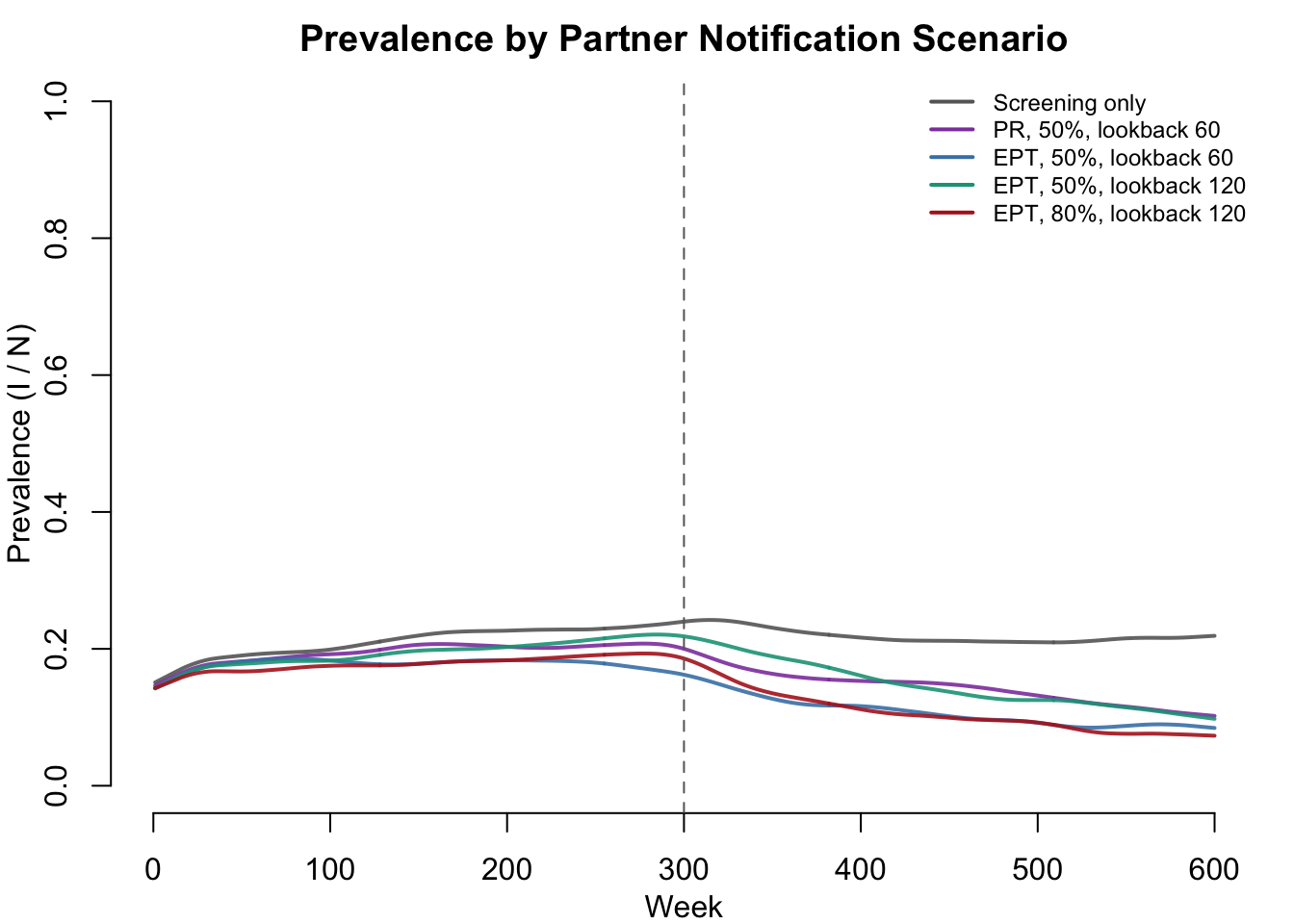

Figure 1: Prevalence over the last three years of the burn-in and the five scenario years, mean of simulations, by partner services strategy. The dashed line marks the last week of the burn-in; the scenarios begin the following week.

Infections averted

alt <- c("none", "pr_6mo", "ept", "ept_cur")
averted <- lapply(alt, function(s) mc_paired(res$pr$inf, res[[s]]$inf))
names(averted) <- alt
added_none <- mc_paired(res$none$inf, res$pr$inf)
ept_window <- mc_paired(res$ept_cur$inf, res$ept$inf)
treated <- sapply(res, function(r) mean(rowSums(r$reach)))
out_tbl <- data.frame(
  Scenario = labels[names(res)],
  `Prevalence after 5 years (%)` = sapply(res, function(r) fmt_ci(mc_mean(r$prev))),
  `New infections` = sapply(res, function(r) round(mean(r$inf))),
  `Infections averted vs patient referral` =
    c(fmt_ci(averted$none, 0), "", sapply(averted[-1], fmt_ci, digits = 0)),
  `Percent change in infections` = sapply(res, function(r)
    round(100 * (mean(r$inf) - mean(res$pr$inf)) / mean(res$pr$inf), 1)),
  `Partners treated` = round(treated),
  `Infections averted per partner treated, vs none` =
    c("", sapply(names(res)[-1], function(s)
      sprintf("%.1f", (mean(res$none$inf) - mean(res[[s]]$inf)) / treated[[s]]))),
  check.names = FALSE, row.names = NULL
)
knitr::kable(out_tbl, caption = "Prevalence in the fifth scenario year (mean of simulations with 95% Monte Carlo interval), new infections over five years, infections averted relative to patient referral (mean of paired differences with 95% Monte Carlo interval; negative values are infections added), the change in infections relative to patient referral, partners treated over five years, and infections averted per partner treated relative to no partner services")

Table 3: Prevalence in the fifth scenario year (mean of simulations with 95% Monte Carlo interval), new infections over five years, infections averted relative to patient referral (mean of paired differences with 95% Monte Carlo interval; negative values are infections added), the change in infections relative to patient referral, partners treated over five years, and infections averted per partner treated relative to no partner services

Scenario	Prevalence after 5 years (%)	New infections	Infections averted vs patient referral	Percent change in infections	Partners treated	Infections averted per partner treated, vs none
No partner services	6.8 (5.7, 7.9)	3792	-1147 (-1461, -833)	43.4	0
Patient referral, 60 days	3.6 (3.0, 4.2)	2645		0.0	420	2.7
Patient referral, 6 months	3.4 (2.8, 4.1)	2574	71 (-188, 330)	-2.7	465	2.6
EPT, 60 days	2.4 (1.7, 3.1)	1994	651 (373, 929)	-24.6	440	4.1
EPT, ongoing partners only	2.6 (1.9, 3.2)	2139	506 (203, 809)	-19.1	421	3.9

par(mfrow = c(1, 1), mar = c(4, 4.5, 3, 1), mgp = c(2.6, 0.8, 0))
short <- c(none = "No partner services", pr_6mo = "PR, 6 months",
           ept = "EPT, 60 days", ept_cur = "EPT, ongoing only")
av <- sapply(averted, function(v) 1000 * v / N)
bp <- barplot(av["est", ], names.arg = short[alt], col = cols[alt],
              ylab = "Infections averted per 1,000 people",
              main = "Five-Year Infections Averted Relative to Patient Referral",
              ylim = range(c(0, av), na.rm = TRUE) * 1.15, cex.names = 0.85)
abline(h = 0)
if (!all(is.na(av["lo", ]))) {
  arrows(bp, av["lo", ], bp, av["hi", ], angle = 90, code = 3, length = 0.04)
}

Figure 2: Infections averted over five years per 1,000 people, relative to patient referral with a 60-day lookback, with 95% Monte Carlo intervals from the paired differences. The bar below zero is the infections added by removing partner services.

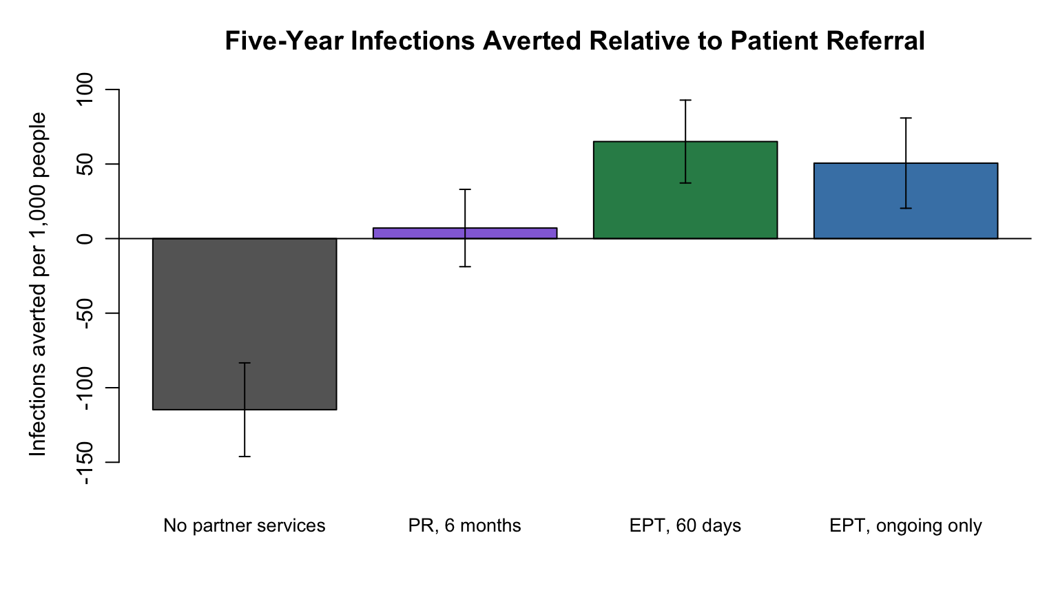
Removing partner services adds 1147 (833, 1461) infections over five years, 43.4% more than under patient referral, and prevalence in the fifth year is 6.8% against 3.6%. The curve without partner services is still rising at year five, so five-year totals understate the long-run difference; the patient referral curve, which continues the burn-in unchanged, drifts within the range of its between-simulation variation (last table). An effect of this size is consistent with the US model of Kretzschmar et al. 2012, in which doubling the share of partners treated reduced positivity as much as tripling screening coverage, and it reflects a system held near its epidemic threshold, where a small change in the number of infections each case causes moves prevalence a long way.

EPT with a 60-day window averts 651 (373, 929) infections relative to patient referral, 24.6% fewer, and EPT for ongoing partners only averts 506 (203, 809), 19.1% fewer. EPT does better although it gives up the chain of diagnosis, because it reaches more partners and treats them a week sooner (next sections). The direction matches the trials. The size is larger than in the Washington State community trial, where chlamydia positivity fell by 11% (prevalence ratio 0.89, 0.77 to 1.04) as the share of index patients given EPT rose from 18% to 34% (Golden et al. 2015), in part because here every index accepts EPT. The ranking can reverse on networks with highly connected people, where tracing through the network finds them (Kao and Enns 2020); the patient referral chain here is short (next sections). The 60-day EPT program reaches the same ongoing partners as the ongoing-only program plus some whose partnerships ended within the window, so its effect should be at least as large. The paired difference, infections under the ongoing-only program minus infections under the 60-day program, is 145 (-90, 380), within Monte Carlo noise; few ended partners are reached, so the two programs differ little, and in one of two further runs with different seeds the ongoing-only program had fewer infections.

Extending patient referral to six months averts 71 (-188, 330) infections, 2.7% fewer than with 60 days, an interval that includes zero. Across this run and two others with different seeds, the change ranged from 11% fewer to 2% more infections, and its interval always included zero. What it adds are partnerships that ended two to six months before diagnosis, which are numerous and rarely reached (next sections). Relative to no partner services, each partner treated averts 2.6 to 4.1 infections over five years, because curing an infected partner also prevents the infections that partner would have caused and the ones those would have caused in turn.

Repeat infection of cured cases

reinf_tbl <- data.frame(
  Scenario = labels[names(res)],
  `Cured cases` = sapply(res, function(r) round(mean(r$tx))),
  `Repeat infection within 13 weeks (%)` = sapply(res, function(r)
    round(100 * sum(r$reinf) / sum(r$tx), 1)),
  `From a partner they already had (%)` = sapply(res, function(r)
    round(100 * sum(r$reinf_prior) / sum(r$reinf))),
  `Relative to patient referral` = sapply(res, function(r)
    round((sum(r$reinf) / sum(r$tx)) / (sum(res$pr$reinf) / sum(res$pr$tx)), 2)),
  check.names = FALSE, row.names = NULL
)
knitr::kable(reinf_tbl, caption = "Cases cured after diagnosis by testing over five years (mean per simulation), the share reinfected within 13 weeks of cure, the share of those repeat infections transmitted by a partner the person already had when cured, and the repeat infection proportion relative to patient referral, pooled over simulations")

Table 4: Cases cured after diagnosis by testing over five years (mean per simulation), the share reinfected within 13 weeks of cure, the share of those repeat infections transmitted by a partner the person already had when cured, and the repeat infection proportion relative to patient referral, pooled over simulations

Scenario	Cured cases	Repeat infection within 13 weeks (%)	From a partner they already had (%)	Relative to patient referral
No partner services	1236	45.0	98	1.41
Patient referral, 60 days	840	31.9	98	1.00
Patient referral, 6 months	826	31.4	98	0.98
EPT, 60 days	651	21.9	97	0.68
EPT, ongoing partners only	706	22.4	97	0.70

par(mfrow = c(1, 1), mar = c(4, 4.5, 3, 1), mgp = c(2.6, 0.8, 0))
reinf <- sapply(res, function(r) {
  100 * c(prior = sum(r$reinf_prior), new = sum(r$reinf - r$reinf_prior)) / sum(r$tx)
})
barplot(reinf, names.arg = c("None", "PR, 60 days", "PR, 6 months",
                             "EPT, 60 days", "EPT, ongoing"),
        col = c("firebrick", "gray75"), cex.names = 0.85,
        ylab = "Reinfected within 13 weeks of cure (%)",
        main = "Repeat Infection of Cured Cases",
        ylim = c(0, max(colSums(reinf)) * 1.3))
legend("topright", fill = c("firebrick", "gray75"), bty = "n", cex = 0.8,
       legend = c("By a partner they had when cured", "By a new partner"))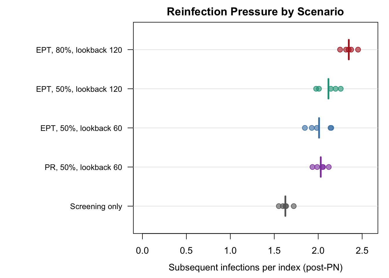

Figure 3: Repeat infection within 13 weeks of cure, by the source of the reinfection: a partner the person already had when cured, or a partner from a partnership that began afterward.

Under patient referral, 31.9% of cured cases are reinfected within 13 weeks, and 98% of those repeat infections come from a partner the person already had when cured; new partners account for few repeat infections within 13 weeks. EPT reduces repeat infection to 21.9%, a ratio of 0.68 to patient referral (0.70 for ongoing partners only). That is close to the relative risks for chlamydia and gonorrhea combined in the Golden trial (0.76, 0.59 to 0.98) and in the Cochrane review against simple patient referral (0.71, 0.56 to 0.89), and a larger reduction than the trials found for chlamydia alone (0.90, 0.60 to 1.35). The absolute levels are about twice those observed (see Simplifications). The six-month lookback leaves repeat infection unchanged, since the partners it adds cannot reinfect the index. A pair model found that treating current partners within three days of the index removes most of the reinfection risk (Low et al. 2014); EPT comes closest to that here because the partner is treated in the same week as the index.

Whom partner services reaches

pn_scn <- c("pr", "pr_6mo", "ept", "ept_cur")
per_index <- function(s, x) sum(x) / sum(res[[s]]$index)
yield_tbl <- data.frame(
  Scenario = labels[pn_scn],
  `Indices per year` = sapply(pn_scn, function(s)
    round(mean(res[[s]]$index) / (horizon / 52))),
  `Partners found per index` = sapply(pn_scn, function(s)
    round(per_index(s, res[[s]]$found), 2)),
  `Ongoing main, casual, ended (%)` = sapply(pn_scn, function(s) {
    paste(round(100 * colSums(res[[s]]$found) / sum(res[[s]]$found)),
          collapse = ", ")
  }),
  `Reached per index` = sapply(pn_scn, function(s)
    round(per_index(s, res[[s]]$reach), 2)),
  `Reached who are infected (%)` = sapply(pn_scn, function(s)
    round(100 * sum(res[[s]]$reach_inf) / sum(res[[s]]$reach))),
  `Infected by type: main, casual, ended (%)` = sapply(pn_scn, function(s) {
    p <- 100 * colSums(res[[s]]$reach_inf) / colSums(res[[s]]$reach)
    paste(ifelse(is.nan(p), "-", round(p)), collapse = ", ")
  }),
  `Partners diagnosed per index` = sapply(pn_scn, function(s)
    round(per_index(s, res[[s]]$part_dx), 2)),
  check.names = FALSE, row.names = NULL
)
knitr::kable(yield_tbl, caption = "Indices handled per year (including partners diagnosed through patient referral), partners found in the lookback window per index (including partners already in care, who are not contacted) and their partnership type, partners reached per index, the share of reached partners who were infected overall and by partnership type, and partners diagnosed per index, pooled over simulations")

Table 5: Indices handled per year (including partners diagnosed through patient referral), partners found in the lookback window per index (including partners already in care, who are not contacted) and their partnership type, partners reached per index, the share of reached partners who were infected overall and by partnership type, and partners diagnosed per index, pooled over simulations

Scenario	Indices per year	Partners found per index	Ongoing main, casual, ended (%)	Reached per index	Reached who are infected (%)	Infected by type: main, casual, ended (%)	Partners diagnosed per index
Patient referral, 60 days	236	1.50	50, 26, 24	0.36	72	78, 61, 48	0.25
Patient referral, 6 months	234	2.01	37, 19, 44	0.40	66	77, 62, 37	0.26
EPT, 60 days	137	1.43	49, 28, 24	0.64	72	76, 65, 49	0.00
EPT, ongoing partners only	149	1.07	64, 36, 0	0.56	74	78, 64, -	0.00

par(mfrow = c(1, 1), mar = c(4, 4.5, 3, 1), mgp = c(2.6, 0.8, 0))
yield <- sapply(pn_scn, function(s) {
  r <- res[[s]]
  c(colSums(r$reach_inf), colSums(r$reach) - colSums(r$reach_inf)) / sum(r$index)
})
ycols <- c("#8e44ad", "#e67e22", "#566573", "#d7bde2", "#f5cba7", "#d5d8dc")
barplot(yield, names.arg = c("PR, 60 days", "PR, 6 months", "EPT, 60 days",
                             "EPT, ongoing only"),
        col = ycols, cex.names = 0.85, ylab = "Partners reached per index",
        main = "Who Partner Services Reaches",
        ylim = c(0, max(colSums(yield)) * 1.45))
legend("top", ncol = 3, bty = "n", fill = ycols[c(1, 4, 2, 5, 3, 6)], cex = 0.75,
       legend = c("Main, infected", "Main, uninfected", "Casual, infected",
                  "Casual, uninfected", "Ended, infected", "Ended, uninfected"))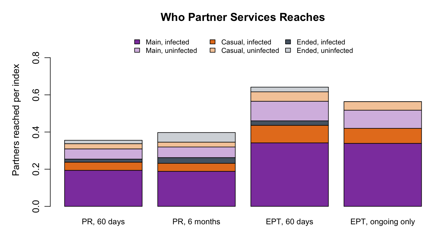

Figure 4: Partners reached per index, by partnership type and infection status when reached.

Patient referral with a 60-day window finds 1.5 partners per index and reaches 0.36; the partners found but not contacted include those already in care, among them the index who referred a partner diagnosed at a PR visit. Index patients in UK clinics named 1.18 to 1.48 partners over a six-month window (Public Health England 2016; Estcourt 2022), fewer than the 2.01 partners per index that the model finds over six months, as expected when not every partner is named. Of the partners found in 60 days, 24% are in partnerships that had already ended, the part of the program that only a partnership history can supply. The six-month window raises that share to 44%: the partners it adds are former partners, who are reached one time in ten and are less often infected. Most of the population effect of partner notification comes from ongoing partners here, as in other models (Althaus et al. 2012; Althaus et al. 2014) and with the small difference between one-month and six-month windows in Weiss et al. 2019.

EPT reaches 0.64 partners per index, 0.28 more than patient referral (the Cochrane review found 0.43 more partners treated per index), and it gives up the 0.25 partners per index who are diagnosed under patient referral and become indices themselves. In a Scottish audit, testing partners and tracing their partners in turn found 22% to 28% more infections than treating partners without testing would have (Forbes and Clutterbuck 2009). Between 66% and 74% of the partners reached are infected, depending on the program, at the top of the published range for current partners and well above the 34% of all notified partners who tested positive in Dutch clinics (van Aar et al. 2018), because the partners reached here are mostly ongoing partners of long standing. Under EPT, 28% of treatments go to uninfected partners, fewer than the 52% to 63% in the EpiModel study of EPT among men who have sex with men (Weiss 2019), for the same reason.

Between-simulation variability

cv_tbl <- data.frame(
  Scenario = labels[names(res)],
  `Mean prevalence after 5 years (%)` = sapply(res, function(r) round(mean(r$prev), 1)),
  `Range across simulations (%)` = sapply(res, function(r)
    sprintf("%.1f to %.1f", min(r$prev), max(r$prev))),
  `CV of five-year infections` = sapply(res, function(r)
    round(sd(r$inf) / mean(r$inf), 2)),
  check.names = FALSE, row.names = NULL
)
knitr::kable(cv_tbl, caption = "Prevalence in the fifth scenario year (mean and range across simulations) and the coefficient of variation of five-year infections, by scenario")

Table 6: Prevalence in the fifth scenario year (mean and range across simulations) and the coefficient of variation of five-year infections, by scenario

Scenario	Mean prevalence after 5 years (%)	Range across simulations (%)	CV of five-year infections
No partner services	6.8	3.3 to 8.3	0.26
Patient referral, 60 days	3.6	2.5 to 4.7	0.26
Patient referral, 6 months	3.4	2.2 to 5.0	0.27
EPT, 60 days	2.4	0.8 to 4.1	0.38
EPT, ongoing partners only	2.6	0.7 to 4.0	0.34

Between-simulation variation is large. Endemic prevalence in a population of 10,000 with a small core group wanders from one simulation to the next, so prevalence five years after the change ranges from 2.5 to 4.7% under patient referral, with a coefficient of variation of five-year infections near 0.26. Resuming a shared burn-in removes the variation that the scenarios share at the moment they resume, but not the divergence that follows, which is why the intervals on infections averted are wide. More simulations narrow the intervals in proportion to the square root of their number, and the run time grows in proportion to the number.

Summary

In this model, patient referral at the level of US practice keeps a chlamydia-like infection endemic at about 3% to 4% prevalence, and removing it raises new infections by 43.4% within five years. EPT lowers infections by a further 24.6% (60-day window) and 19.1% (ongoing partners only) and lowers repeat infection of cured cases by about 32% relative to patient referral, despite ending the chain of diagnosis, because it reaches more partners and reaches them sooner. A six-month lookback finds many more partners, mostly former ones, and lowers infections by 2.7%, with an interval that includes zero. Nearly every repeat infection comes from a partner the person already had when cured, which is the failure partner notification exists to prevent.

Next Steps

• Abstinence until partners are treated. In infect, drop the discordant pairs in which one partner is a cured index still within an abstinence window and the other is an ongoing partner who has not been treated. In the Golden trial, 88% of women with chlamydia reported no sex with an untreated partner; the change should bring repeat infection toward the observed range and shows how much of partner notification’s benefit survives a realistic behavioral response.
• Offer EPT and fall back to PR. Draw each index’s acceptance of EPT (a median of 65% in Layton 2020) and send the partners of indices who decline down the PR path. This is how EPT is delivered, and it turns the EPT scenarios from upper bounds into estimates.
• The most recent partner. CDC guidance also notifies the most recent partner when the last partnership ended before the 60-day window. Call get_partners() with a longer truncate (and raise truncate.el.cuml to match), keep, for each index with no partner in the window, the row with the latest stop, and treat that partner.
• Retesting at three months. Schedule a test at tx.time + 13 for a share of cured cases. Repeat infections are then found and treated, and each one starts a new round of partner notification.
• Test before treating. Treat reached partners only if they test positive, as the 2026 BASHH guideline does for late-presenting asymptomatic contacts, and count the treatments saved against the infections missed.
• Age structure and asymmetric transmission. Add age groups with age-disparate mixing and a higher male-to-female transmission probability. Both should raise prevalence in young women relative to young men toward the NHANES pattern.
• Costs. The partners treated and infections averted here are the inputs of a cost-effectiveness analysis; the cost-effectiveness example shows how to attach costs and quality-adjusted life years to an EpiModel simulation.

References

Partner notification guidance, trials, and program data:

• Workowski KA, Bachmann LH, Chan PA, et al. (2021). Sexually transmitted infections treatment guidelines, 2021. MMWR Recomm Rep 70(4):1-187. https://doi.org/10.15585/mmwr.rr7004a1
• Centers for Disease Control and Prevention. (2006). Expedited partner therapy in the management of sexually transmitted diseases: review and guidance. https://stacks.cdc.gov/view/cdc/6804
• McClean H, Radcliffe K, Sullivan A, Ahmed-Jushuf I. (2013). 2012 BASHH statement on partner notification for sexually transmissible infections. Int J STD AIDS 24(4):253-261. https://doi.org/10.1177/0956462412472804
• Saunders J, Burley N, Brice S, et al. (2026). British Association for Sexual Health and HIV UK national guideline for the management of infection with Chlamydia trachomatis, 2026. Int J STD AIDS, published online August 24, 2026. https://doi.org/10.1177/09564624261475950
• Schillinger JA, Kissinger P, Calvet H, et al. (2003). Patient-delivered partner treatment with azithromycin to prevent repeated Chlamydia trachomatis infection among women: a randomized, controlled trial. Sex Transm Dis 30(1):49-56. https://doi.org/10.1097/00007435-200301000-00011
• Golden MR, Whittington WLH, Handsfield HH, et al. (2005). Effect of expedited treatment of sex partners on recurrent or persistent gonorrhea or chlamydial infection. N Engl J Med 352(7):676-685. https://doi.org/10.1056/NEJMoa041681
• Kissinger P, Mohammed H, Richardson-Alston G, et al. (2005). Patient-delivered partner treatment for male urethritis: a randomized, controlled trial. Clin Infect Dis 41(5):623-629. https://doi.org/10.1086/432476
• Ferreira A, Young T, Mathews C, Zunza M, Low N. (2013). Strategies for partner notification for sexually transmitted infections, including HIV. Cochrane Database Syst Rev (10):CD002843. https://doi.org/10.1002/14651858.CD002843.pub2
• Estcourt CS, Stirrup O, Copas A, et al. (2022). Accelerated partner therapy contact tracing for people with chlamydia (LUSTRUM): a crossover cluster-randomised controlled trial. Lancet Public Health 7(10):e853-e865. https://doi.org/10.1016/S2468-2667(22)00204-3
• Golden MR, Kerani RP, Stenger M, et al. (2015). Uptake and population-level impact of expedited partner therapy (EPT) on Chlamydia trachomatis and Neisseria gonorrhoeae: the Washington State community-level randomized trial of EPT. PLoS Med 12(1):e1001777. https://doi.org/10.1371/journal.pmed.1001777
• Public Health England. (2016). Partner notification in chlamydia screening: national audit report. https://assets.publishing.service.gov.uk/media/5b80052fed915d74f2d4c70b/NCSP_PN_audit_report_FINAL.pdf
• Estcourt CS, Flowers P, Cassell JA, et al. (2022). Going beyond ‘regular and casual’: development of a classification of sexual partner types to enhance partner notification for STIs. Sex Transm Infect 98(2):108-114. https://doi.org/10.1136/sextrans-2020-054846
• Layton E, Vaisey A, Goller JL, et al. (2020). The views of patients and partners toward patient-delivered partner therapy for chlamydia: a systematic review. Sex Transm Dis 47(12):790-797. https://doi.org/10.1097/OLQ.0000000000001260
• Golden MR, Hogben M, Handsfield HH, et al. (2003). Partner notification for HIV and STD in the United States: low coverage for gonorrhea, chlamydial infection, and HIV. Sex Transm Dis 30(6):490-496. https://doi.org/10.1097/00007435-200306000-00004
• Patel HC, Viswalingam ND, Goh BT. (1994). Chlamydial ocular infection: efficacy of partner notification by patient referral. Int J STD AIDS 5(4):244-247. https://doi.org/10.1177/095646249400500403
• McMahon BL, Buitendam E, Symonds M, Estcourt CS, Saunders J. (2025). Use of a five-category partner-type classification within a chlamydia and gonorrhoea service evaluation highlights opportunities for targeted partner notification to improve STI control. Sex Transm Infect 101(1):55-58. https://doi.org/10.1136/sextrans-2024-056108
• Forbes G, Clutterbuck DJ. (2009). How many cases of chlamydial infection would we miss by not testing partners for infection? Int J STD AIDS 20(4):267-268. https://doi.org/10.1258/ijsa.2008.008387
• van Aar F, van Benthem BHB, van den Broek IVF, Götz HM. (2018). STIs in sex partners notified for chlamydia exposure: implications for expedited partner therapy. Sex Transm Infect 94(8):619-621. https://doi.org/10.1136/sextrans-2017-053364

Models of chlamydia and partner notification:

• Yorke JA, Hethcote HW, Nold A. (1978). Dynamics and control of the transmission of gonorrhea. Sex Transm Dis 5(2):51-56. https://doi.org/10.1097/00007435-197804000-00003
• Kretzschmar M, van Duynhoven YT, Severijnen AJ. (1996). Modeling prevention strategies for gonorrhea and Chlamydia using stochastic network simulations. Am J Epidemiol 144(3):306-317. https://doi.org/10.1093/oxfordjournals.aje.a008926
• Turner KME, Adams EJ, Gay N, Ghani AC, Mercer C, Edmunds WJ. (2006). Developing a realistic sexual network model of chlamydia transmission in Britain. Theor Biol Med Model 3:3. https://doi.org/10.1186/1742-4682-3-3
• Althaus CL, Heijne JCM, Roellin A, Low N. (2010). Transmission dynamics of Chlamydia trachomatis affect the impact of screening programmes. Epidemics 2(3):123-131. https://doi.org/10.1016/j.epidem.2010.04.002
• Heijne JCM, Althaus CL, Herzog SA, Kretzschmar M, Low N. (2011). The role of reinfection and partner notification in the efficacy of Chlamydia screening programs. J Infect Dis 203(3):372-377. https://doi.org/10.1093/infdis/jiq050
• Althaus CL, Heijne JCM, Herzog SA, Roellin A, Low N. (2012). Individual and population level effects of partner notification for Chlamydia trachomatis. PLoS One 7(12):e51438. https://doi.org/10.1371/journal.pone.0051438
• Kretzschmar M, Satterwhite C, Leichliter J, Berman S. (2012). Effects of screening and partner notification on Chlamydia positivity in the United States: a modeling study. Sex Transm Dis 39(5):325-331. https://doi.org/10.1097/OLQ.0b013e31824e52c2
• Althaus CL, Turner KME, Mercer CH, et al. (2014). Effectiveness and cost-effectiveness of traditional and new partner notification technologies for curable sexually transmitted infections: observational study, systematic reviews and mathematical modelling. Health Technol Assess 18(2):1-100. https://doi.org/10.3310/hta18020
• Low N, Heijne JCM, Herzog SA, Althaus CL. (2014). Reinfection by untreated partners of people treated for Chlamydia trachomatis and Neisseria gonorrhoeae: mathematical modelling study. Sex Transm Infect 90(3):254-256. https://doi.org/10.1136/sextrans-2013-051279
• Weiss KM, Jones JS, Katz DA, et al. (2019). Epidemiological impact of expedited partner therapy for men who have sex with men: a modeling study. Sex Transm Dis 46(11):697-705. https://doi.org/10.1097/OLQ.0000000000001058
• Kao SZ, Enns EA. (2020). Follow the sex: influence of network structure on the effectiveness and cost-effectiveness of partner management strategies for sexually transmitted infection control. Sex Transm Dis 47(2):71-79. https://doi.org/10.1097/OLQ.0000000000001100

Natural history, transmission, and epidemiology:

• Lewis J, Price MJ, Horner PJ, White PJ. (2017). Genital Chlamydia trachomatis infections clear more slowly in men than women, but are less likely to become established. J Infect Dis 216(2):237-244. https://doi.org/10.1093/infdis/jix283
• Davies B, Anderson SJ, Turner KME, Ward H. (2014). How robust are the natural history parameters used in chlamydia transmission dynamic models? A systematic review. Theor Biol Med Model 11:8. https://doi.org/10.1186/1742-4682-11-8
• Farley TA, Cohen DA, Elkins W. (2003). Asymptomatic sexually transmitted diseases: the case for screening. Prev Med 36(4):502-509. https://doi.org/10.1016/s0091-7435(02)00058-0
• Quinn TC, Gaydos C, Shepherd M, et al. (1996). Epidemiologic and microbiologic correlates of Chlamydia trachomatis infection in sexual partnerships. JAMA 276(21):1737-1742. PMID 8940322.
• Althaus CL, Heijne JCM, Low N. (2012). Towards more robust estimates of the transmissibility of Chlamydia trachomatis. Sex Transm Dis 39(5):402-404. https://doi.org/10.1097/OLQ.0b013e318248a550
• Lewis J, White PJ, Price MJ. (2021). Per-partnership transmission probabilities for Chlamydia trachomatis infection: evidence synthesis of population-based survey data. Int J Epidemiol 50(2):510-517. https://doi.org/10.1093/ije/dyaa202
• Rogers SM, Miller WC, Turner CF, et al. (2008). Concordance of Chlamydia trachomatis infections within sexual partnerships. Sex Transm Infect 84(1):23-28. https://doi.org/10.1136/sti.2007.027029
• Torrone E, Papp J, Weinstock H. (2014). Prevalence of Chlamydia trachomatis genital infection among persons aged 14-39 years, United States, 2007-2012. MMWR Morb Mortal Wkly Rep 63(38):834-838. PMID 25254560.
• Kreisel KM, Weston EJ, St Cyr SB, Spicknall IH. (2021). Estimates of the prevalence and incidence of chlamydia and gonorrhea among US men and women, 2018. Sex Transm Dis 48(4):222-231. https://doi.org/10.1097/OLQ.0000000000001382
• Centers for Disease Control and Prevention. (2024). Sexually transmitted infections surveillance, 2023. https://stacks.cdc.gov/view/cdc/255132
• Pazol K, Robbins CL, Black LI, et al. (2017). Receipt of selected preventive health services for women and men of reproductive age, United States, 2011-2013. MMWR Surveill Summ 66(20):1-31. https://doi.org/10.15585/mmwr.ss6620a1
• He L, Patel C, Tao G. (2023). National chlamydia screening rate in young sexually active women using HEDIS measures in the United States, 2011 to 2020. Sex Transm Dis 50(7):415-419. https://doi.org/10.1097/OLQ.0000000000001809
• Geisler WM, Uniyal A, Lee JY, et al. (2015). Azithromycin versus doxycycline for urogenital Chlamydia trachomatis infection. N Engl J Med 373(26):2512-2521. https://doi.org/10.1056/NEJMoa1502599
• Kong FYS, Tabrizi SN, Law M, et al. (2014). Azithromycin versus doxycycline for the treatment of genital chlamydia infection: a meta-analysis of randomized controlled trials. Clin Infect Dis 59(2):193-205. https://doi.org/10.1093/cid/ciu220
• Hosenfeld CB, Workowski KA, Berman S, et al. (2009). Repeat infection with chlamydia and gonorrhea among females: a systematic review of the literature. Sex Transm Dis 36(8):478-489. https://doi.org/10.1097/OLQ.0b013e3181a2a933
• Fung M, Scott KC, Kent CK, Klausner JD. (2007). Chlamydial and gonococcal reinfection among men: a systematic review of data to evaluate the need for retesting. Sex Transm Infect 83(4):304-309. https://doi.org/10.1136/sti.2006.024059
• Mercer CH, Tanton C, Prah P, et al. (2013). Changes in sexual attitudes and lifestyles in Britain through the life course and over time: findings from the National Surveys of Sexual Attitudes and Lifestyles (Natsal). Lancet 382(9907):1781-1794. https://doi.org/10.1016/S0140-6736(13)62035-8
• Chandra A, Mosher WD, Copen C, Sionean C. (2011). Sexual behavior, sexual attraction, and sexual identity in the United States: data from the 2006-2008 National Survey of Family Growth. Natl Health Stat Report (36):1-36. https://www.cdc.gov/nchs/data/nhsr/nhsr036.pdf
• Burington B, Hughes JP, Whittington WLH, et al. (2010). Estimating duration in partnership studies: issues, methods and examples. Sex Transm Infect 86(2):84-89. https://doi.org/10.1136/sti.2009.037960

The network structure, transmission probability, testing rates, and reach probabilities are illustrative choices, selected to place the model in a plausible endemic regime for young heterosexual adults and to reproduce the published targets in the calibration table. They are not calibrated to any population.

Author

Samuel M. Jenness, Emory University