SEIR Model with All-or-Nothing Vaccination

Binary vaccine immunity, herd immunity effects, and multi-route vaccination in a dynamic network

SEIR

vaccination

vital dynamics

herd immunity

intermediate

SEIR epidemic model with all-or-nothing vaccination through three delivery routes — initial coverage, ongoing campaigns, and newborn vaccination — over a dynamic network with vital dynamics.

Author

Connor M. Van Meter

Published

October 1, 2018

Overview

This example demonstrates how to model an all-or-nothing (AON) vaccination intervention on an SEIR epidemic spreading over a dynamic network with vital dynamics (births and deaths). In an AON vaccine model, vaccinated individuals are either fully immune or completely unprotected — there is no partial reduction in susceptibility. This is a reasonable approximation for vaccines where the immune response is binary: either sterilizing immunity is achieved or it is not.

The key extension is a vaccination cascade operating through three routes: initial population coverage at the start of the simulation, ongoing vaccination campaigns among the existing population, and vaccination of newborns at arrival. Protected individuals are moved to a separate “V” (vaccine-immune) compartment and cannot be infected. As the V compartment grows, it reduces the pool of susceptible individuals available for transmission, creating herd immunity effects — even unvaccinated susceptibles benefit as the infectious pool shrinks.

This example introduces several important EpiModel techniques: adding custom node attributes for vaccination and protection status, implementing a separate initialization module, modeling vaccination at multiple population entry points, and comparing disease dynamics across scenarios with and without intervention. We run two scenarios — a baseline with no vaccination and a strong AON vaccination program — to illustrate how binary vaccine protection translates into population-level epidemic control.

Download the Code

The standalone R scripts for this example are available for download:

model.R — Main simulation script with network estimation, scenario comparison, and analysis
module-fx.R — Custom module functions for vaccination, infection, progression, departures, and arrivals

Model Structure

The model extends the standard SEIR framework with a vaccine-immune compartment (V) and vital dynamics:

Compartment	Label	Description
Susceptible	S	Not infected; at risk of infection
Exposed	E	Infected but not yet infectious (latent period)
Infectious	I	Infected and capable of transmitting
Recovered	R	Recovered with permanent natural immunity
Vaccine-Immune	V	Protected by AON vaccination; completely immune

flowchart TD
    in(( )) -->|"arrival"| S
    in -->|"vaccinated &<br/>protected"| V

    S["<b>S</b><br/>Susceptible"] -->|"infection<br/>(se.flow)"| E["<b>E</b><br/>Exposed"]
    S -->|"vaccination<br/>campaign"| V["<b>V</b><br/>Vaccine-Immune"]
    E -->|"progression<br/>(ei.rate)"| I["<b>I</b><br/>Infectious"]
    I -->|"recovery<br/>(ir.rate)"| R["<b>R</b><br/>Recovered"]

    S -->|"departure"| out1(( ))
    E -->|"departure"| out2(( ))
    I -->|"departure<br/>(elevated)"| out3(( ))
    R -->|"departure"| out4(( ))
    V -->|"departure"| out5(( ))

    style S fill:#3498db,color:#fff
    style E fill:#f39c12,color:#fff
    style I fill:#e74c3c,color:#fff
    style R fill:#27ae60,color:#fff
    style V fill:#8e44ad,color:#fff
    style in fill:none,stroke:none
    style out1 fill:none,stroke:none
    style out2 fill:none,stroke:none
    style out3 fill:none,stroke:none
    style out4 fill:none,stroke:none
    style out5 fill:none,stroke:none

SEIR-V model flow diagram. Susceptibles may become infected (S to E) or vaccinated (S to V). Arrivals enter as S or V depending on newborn vaccination. All compartments face background departures, with elevated mortality for the infectious.

All-or-Nothing Vaccination Mechanism

The AON vaccine works in two steps. First, an individual receives the vaccine (tracked by the vaccination attribute, which records the route: “initial”, “progress”, or “arrival”). Second, a vaccinated susceptible individual has a probability of receiving protection. If protected, they move to status = "v" and become completely immune. If not protected, they remain susceptible with protection = "none" and cannot be re-vaccinated.

Key assumptions of this model:

Binary immunity: Protected individuals have 100% immunity (cannot be infected). Unprotected individuals receive 0% benefit.
One-shot vaccination: Individuals can only be vaccinated once. Those who fail to receive protection on their first vaccination do not get a second chance.
No waning: Vaccine immunity is permanent. Protected individuals remain in V indefinitely.

Vaccination Routes

Route	When	Rate Parameters
Initialization	Timestep 2 only	`vaccination.rate.initialization`, `protection.rate.initialization`
Progression	Every timestep	`vaccination.rate.progression`, `protection.rate.progression`
Arrivals	At birth	`vaccination.rate.arrivals`, `protection.rate.arrivals`

The effective per-route protection rate is the product of the two rates. For example, with vaccination.rate.arrivals = 0.6 and protection.rate.arrivals = 0.8, 48% of newborns become vaccine-immune.

Setup

library(EpiModel)

We set simulation parameters for the interactive session. Five simulations over 500 weekly timesteps provide enough replication and duration to observe the epidemic trajectory and herd immunity effects.

nsims <- 5
ncores <- 5
nsteps <- 500

Custom Modules

This model uses five custom module functions. The vaccine attribute initialization module runs once to set up vaccination tracking, the infection module handles S-to-E transmission, the progression module moves individuals through E-to-I and I-to-R, the departure module simulates mortality, and the arrival module handles births and ongoing vaccination.

Vaccine Attribute Initialization (`init_vaccine_attrs`)

This module runs once at the first module call to initialize the vaccination and protection attributes for all nodes. It checks whether attributes have already been set using override.null.error and stochastically vaccinates the initial population with the initialization rates. Only vaccinated susceptible individuals can receive protection — vaccinated nodes that are already infected gain no benefit.

init_vaccine_attrs <- function(dat, at) {

1  if (is.null(get_attr(dat, "vaccination", override.null.error = TRUE))) {

    ## Attributes ##
    active <- get_attr(dat, "active")
    n <- sum(active == 1)
    status <- get_attr(dat, "status")

    ## Parameters ##
    vaccination.rate.init <- get_param(dat, "vaccination.rate.initialization")
    protection.rate.init <- get_param(dat, "protection.rate.initialization")

    ## Initialize vectors (NA = unvaccinated/unprotected) ##
    vaccination <- rep(NA, n)
    protection <- rep(NA, n)

    ## Stochastic vaccination of initial population ##
    idsEligVacInit <- which(active == 1)
    vecVacInit <- rbinom(length(idsEligVacInit), 1, vaccination.rate.init)
    idsVacInit <- idsEligVacInit[which(vecVacInit == 1)]
    vaccination[idsVacInit] <- "initial"

    ## Stochastic protection among vaccinated susceptibles ##
2    idsEligProtInit <- which(vaccination == "initial" & status == "s")
    vecProtInit <- rbinom(length(idsEligProtInit), 1, protection.rate.init)
    idsProtInit <- idsEligProtInit[which(vecProtInit == 1)]
    idsNoProtInit <- setdiff(idsVacInit, idsProtInit)
    protection[idsProtInit] <- "initial"
3    protection[idsNoProtInit] <- "none"

    ## Write out attributes ##
    dat <- set_attr(dat, "vaccination", vaccination)
    dat <- set_attr(dat, "protection", protection)
  }

  return(dat)
}

1: override.null.error = TRUE returns NULL instead of an error if the attribute does not exist yet, allowing this module to detect its first call and run initialization exactly once.
2: Only vaccinated susceptible nodes are eligible for protection. Individuals who are already infected at initialization gain no benefit from vaccination.
3: Vaccinated but unprotected individuals receive protection = "none", which permanently marks them as ineligible for future vaccination — this enforces the one-shot assumption.

Infection Module (`infect`)

This module simulates S-to-E transmission along discordant edges in the network. The critical feature for the vaccination model is that protected individuals (status = "v") are automatically excluded from the susceptible pool by discord_edgelist(), which only considers nodes with status = "s" as susceptible. No special vaccination logic is needed in the infection module itself.

infect <- function(dat, at) {

  ## Attributes ##
  active <- get_attr(dat, "active")
  status <- get_attr(dat, "status")
  infTime <- get_attr(dat, "infTime")

  ## Parameters ##
  inf.prob <- get_param(dat, "inf.prob")
  act.rate <- get_param(dat, "act.rate")

  ## Find infected nodes ##
  idsInf <- which(active == 1 & status == "i")
  nActive <- sum(active == 1)
  nElig <- length(idsInf)

  ## Initialize incidence counter ##
  nInf <- 0

  ## Transmission process ##
  if (nElig > 0 && nElig < nActive) {

1    del <- discord_edgelist(dat, at)

    if (!(is.null(del)) && nrow(del) > 0) {

      del$transProb <- inf.prob
      del$actRate <- act.rate
2      del$finalProb <- 1 - (1 - del$transProb)^del$actRate

      transmit <- rbinom(nrow(del), 1, del$finalProb)
      del <- del[which(transmit == 1), ]

      idsNewInf <- unique(del$sus)
      nInf <- length(idsNewInf)

      if (nInf > 0) {
3        status[idsNewInf] <- "e"
        dat <- set_attr(dat, "status", status)
        infTime[idsNewInf] <- at
        dat <- set_attr(dat, "infTime", infTime)
      }
    }
  }

  ## Summary statistics ##
  dat <- set_epi(dat, "se.flow", at, nInf)

  dat <- set_epi(dat, "s.num", at, sum(active == 1 & status == "s"))
  dat <- set_epi(dat, "e.num", at, sum(active == 1 & status == "e"))
  dat <- set_epi(dat, "i.num", at, sum(active == 1 & status == "i"))
  dat <- set_epi(dat, "r.num", at, sum(active == 1 & status == "r"))
4  dat <- set_epi(dat, "v.num", at, sum(active == 1 & status == "v"))

  return(dat)
}

1: discord_edgelist() returns edges connecting infectious and susceptible nodes. Vaccine-immune nodes (status = "v") are not considered susceptible, so they never appear on this list — this is the mechanism by which AON vaccination prevents infection.
2: The per-timestep transmission probability accounts for multiple acts per partnership: \(P = 1 - (1 - p)^a\) where \(p\) is the per-act probability and \(a\) is the act rate.
3: Newly infected individuals enter the exposed (E) compartment, not directly infectious — they must progress through the latent period before they can transmit.
4: The V compartment count is tracked alongside the standard SEIR compartments so it can be plotted and analyzed.

Disease Progression Module (`progress`)

This module handles E-to-I progression (exposed to infectious) and I-to-R recovery (infectious to recovered). There is no R-to-S transition — this is an SEIR model with permanent natural immunity after recovery.

progress <- function(dat, at) {

  ## Attributes ##
  active <- get_attr(dat, "active")
  status <- get_attr(dat, "status")

  ## Parameters ##
  ei.rate <- get_param(dat, "ei.rate")
  ir.rate <- get_param(dat, "ir.rate")

  ## E -> I (exposed to infectious) ##
  nProg <- 0
  idsEligProg <- which(active == 1 & status == "e")
  nEligProg <- length(idsEligProg)

  if (nEligProg > 0) {
1    vecProg <- which(rbinom(nEligProg, 1, ei.rate) == 1)
    if (length(vecProg) > 0) {
      idsProg <- idsEligProg[vecProg]
      nProg <- length(idsProg)
      status[idsProg] <- "i"
    }
  }

  ## I -> R (infectious to recovered) ##
  nRec <- 0
  idsEligRec <- which(active == 1 & status == "i")
  nEligRec <- length(idsEligRec)

  if (nEligRec > 0) {
    vecRec <- which(rbinom(nEligRec, 1, ir.rate) == 1)
    if (length(vecRec) > 0) {
      idsRec <- idsEligRec[vecRec]
      nRec <- length(idsRec)
      status[idsRec] <- "r"
    }
  }

  ## Write out updated status ##
  dat <- set_attr(dat, "status", status)

  ## Summary statistics ##
  dat <- set_epi(dat, "ei.flow", at, nProg)
  dat <- set_epi(dat, "ir.flow", at, nRec)

  return(dat)
}

1: Each exposed individual faces an independent Bernoulli trial with probability ei.rate at each timestep. With ei.rate = 0.05, the mean latent period is \(1/0.05 = 20\) weeks. The same geometric waiting time applies to I-to-R recovery.

Departure Module (`dfunc`)

This module simulates mortality (departures) with disease-induced excess. All active nodes face a baseline departure.rate per timestep, while infected individuals (status “i”) have their rate multiplied by departure.disease.mult, representing excess disease-induced mortality.

dfunc <- function(dat, at) {

  ## Attributes ##
  active <- get_attr(dat, "active")
  status <- get_attr(dat, "status")
  exitTime <- get_attr(dat, "exitTime")

  ## Parameters ##
  departure.rate <- get_param(dat, "departure.rate")
  dep.rates <- rep(departure.rate, length(active))
  dep.dis.mult <- get_param(dat, "departure.disease.mult")

  ## Determine eligible (alive) nodes ##
  idsElig <- which(active == 1)
  nElig <- length(idsElig)
  nDeaths <- 0

  if (nElig > 0) {

    dep_rates_of_elig <- dep.rates[idsElig]

    idsElig.inf <- which(status[idsElig] == "i")
1    dep_rates_of_elig[idsElig.inf] <- dep.rates[idsElig.inf] * dep.dis.mult

    ## Stochastic departure process ##
    vecDeaths <- which(rbinom(nElig, 1, dep_rates_of_elig) == 1)
    idsDeaths <- idsElig[vecDeaths]
    nDeaths <- length(idsDeaths)

    if (nDeaths > 0) {
      active[idsDeaths] <- 0
2      exitTime[idsDeaths] <- at
    }
  }

  ## Write out updated attributes ##
  dat <- set_attr(dat, "active", active)
  dat <- set_attr(dat, "exitTime", exitTime)

  ## Summary statistics ##
  dat <- set_epi(dat, "d.flow", at, nDeaths)

  return(dat)
}

1: Infected individuals face departure.rate * departure.disease.mult (2x baseline), representing excess disease-induced mortality. This creates selective pressure that removes infectious individuals faster than other compartments.
2: Setting exitTime records when each node departs, which EpiModel uses for network bookkeeping and summary statistics.

Arrival Module (`afunc`)

This is the most complex module, handling both births (new node arrivals) and ongoing vaccination. Two vaccination routes operate each timestep: progression (campaigns among existing unvaccinated nodes) and arrivals (newborn vaccination). After all vaccination processing, any susceptible node with vaccine protection is moved to status = "v".

afunc <- function(dat, at) {

  ## Attributes ##
  active <- get_attr(dat, "active")
  status <- get_attr(dat, "status")
  infTime <- get_attr(dat, "infTime")

  ## Parameters ##
  nActive <- sum(active == 1)
  nTotal <- length(active)
  a.rate <- get_param(dat, "arrival.rate")
  vaccination.rate.arrivals <- get_param(dat, "vaccination.rate.arrivals")
  protection.rate.arrivals <- get_param(dat, "protection.rate.arrivals")
  vaccination.rate.progression <- get_param(dat, "vaccination.rate.progression")
  protection.rate.progression <- get_param(dat, "protection.rate.progression")

  ## Initialize flow counters ##
  nVax.prog <- 0
  nPrt.prog <- 0
  nVax.arrival <- 0
  nPrt.arrival <- 0

  vaccination <- get_attr(dat, "vaccination")
  protection <- get_attr(dat, "protection")

  ## --- VACCINATION PROGRESSION --- ##
1  idsEligVacProg <- which(is.na(vaccination) & active == 1)
  vecVacProg <- rbinom(length(idsEligVacProg), 1, vaccination.rate.progression)
  idsVacProg <- idsEligVacProg[which(vecVacProg == 1)]
  vaccination[idsVacProg] <- "progress"

  idsEligProtProg <- which(vaccination == "progress" & is.na(protection) & status == "s")
  vecProtProg <- rbinom(length(idsEligProtProg), 1, protection.rate.progression)
  idsProtProg <- idsEligProtProg[which(vecProtProg == 1)]
  idsNoProtProg <- setdiff(idsVacProg, idsProtProg)
  protection[idsProtProg] <- "progress"
  protection[idsNoProtProg] <- "none"

  nVax.prog <- length(idsVacProg)
  nPrt.prog <- length(idsProtProg)

  ## --- ARRIVAL PROCESS --- ##
  nArrivalsExp <- nActive * a.rate
2  nArrivals <- rpois(1, nArrivalsExp)

  if (nArrivals > 0) {
3    dat <- append_core_attr(dat, at, nArrivals)

    newNodes <- (nTotal + 1):(nTotal + nArrivals)
    status <- c(status, rep("s", nArrivals))
    infTime <- c(infTime, rep(NA, nArrivals))
    vaccination <- c(vaccination, rep(NA, nArrivals))
    protection <- c(protection, rep(NA, nArrivals))

    # Vaccinate new arrivals
    vaccinatedNewArrivals <- rbinom(nArrivals, 1, vaccination.rate.arrivals)
    vaccination[newNodes] <- ifelse(vaccinatedNewArrivals == 1, "arrival", NA)
    nVax.arrival <- sum(vaccinatedNewArrivals == 1)

    # Confer protection to vaccinated susceptible arrivals
    idsEligProtArrival <- which(
      vaccination == "arrival" & status == "s" & is.na(protection)
    )
    vecProtArrival <- rbinom(length(idsEligProtArrival), 1, protection.rate.arrivals)
    idsProtArrival <- idsEligProtArrival[which(vecProtArrival == 1)]
    idsNoProtArrival <- idsEligProtArrival[which(vecProtArrival == 0)]
    protection[idsProtArrival] <- "arrival"
    protection[idsNoProtArrival] <- "none"
    nPrt.arrival <- sum(vecProtArrival == 1)
  }

  ## --- UPDATE STATUS: protected susceptibles -> vaccine-immune --- ##
  active <- get_attr(dat, "active")
  statusV <- which(
    status == "s" & protection %in% c("initial", "progress", "arrival") &
      active == 1
  )
4  status[statusV] <- "v"

  ## Write out updated attributes ##
  dat <- set_attr(dat, "status", status)
  dat <- set_attr(dat, "vaccination", vaccination)
  dat <- set_attr(dat, "protection", protection)
  dat <- set_attr(dat, "infTime", infTime)

  ## Summary statistics ##
  dat <- set_epi(dat, "a.flow", at, nArrivals)
  dat <- set_epi(dat, "vac.flow", at, nVax.prog + nVax.arrival)
  dat <- set_epi(dat, "prt.flow", at, nPrt.prog + nPrt.arrival)
  dat <- set_epi(dat, "vac.num", at,
                 sum(active == 1 & vaccination %in%
                       c("initial", "progress", "arrival"), na.rm = TRUE))
  dat <- set_epi(dat, "prt.num", at,
                 sum(active == 1 & protection %in%
                       c("initial", "progress", "arrival"), na.rm = TRUE))

  return(dat)
}

1: Only unvaccinated (is.na(vaccination)) active nodes are eligible for campaign vaccination. This enforces the one-shot rule — previously vaccinated individuals (whether protected or not) cannot be re-vaccinated.
2: The number of arrivals is drawn from a Poisson distribution with mean nActive * arrival.rate, producing stochastic variation in births each week.
3: append_core_attr() is the EpiModel function for adding new nodes to the simulation, initializing their core attributes (active status, unique ID, entry time).
4: This is the all-or-nothing mechanism: any susceptible node with vaccine protection is moved to status = "v" (complete immunity). After this step, discord_edgelist() in the infection module will never consider these nodes as susceptible.

Network Model

We initialize a 500-node network with a simple edges-only formation model targeting a mean degree of 0.8 (200 edges). The dissolution coefficient is adjusted for population turnover using the departure rate.

n <- 500
nw <- network_initialize(n)

formation <- ~edges
mean_degree <- 0.8
n_edges <- mean_degree * (n / 2)
target.stats <- c(n_edges)

The departure rate of 0.008 per week corresponds to a mean lifespan of approximately 2.4 years. This is high relative to real human populations but creates visible demographic turnover within the simulation window, demonstrating how vital dynamics interact with vaccination and disease transmission. The dissolution coefficient accounts for this turnover so that the target partnership duration of 50 weeks is maintained in the open population.

departure_rate <- 0.008

coef.diss <- dissolution_coefs(
  dissolution = ~offset(edges),
  duration = 50,
1  d.rate = departure_rate
)
coef.diss

1: Including d.rate adjusts the dissolution coefficient for population turnover. Without this correction, partnerships would dissolve faster than intended because node departures also end partnerships.

Dissolution Coefficients
=======================
Dissolution Model: ~offset(edges)
Target Statistics: 50
Crude Coefficient: 3.89182
Mortality/Exit Rate: 0.008
Adjusted Coefficient: 5.485385

Network Estimation

est <- netest(nw, formation, target.stats, coef.diss)

Network Diagnostics

We simulate from the fitted network model to verify it reproduces the target statistics. The diagnostics check that the mean number of edges remains near 200 and that the degree distribution is stable.

dx <- netdx(est, nsims = nsims, ncores = ncores, nsteps = nsteps,
            nwstats.formula = ~edges + isolates + degree(0:5))


Network Diagnostics
-----------------------
- Simulating 5 networks
- Calculating formation statistics

print(dx)

EpiModel Network Diagnostics
=======================
Diagnostic Method: Dynamic
Simulations: 5
Time Steps per Sim: 500

Formation Diagnostics
----------------------- 
         Target Sim Mean Pct Diff Sim SE Z Score SD(Sim Means) SD(Statistic)
edges       200  199.111   -0.445  2.411  -0.369         1.956        13.711
isolates     NA  224.125       NA  2.481      NA         1.473        14.747
degree0      NA  224.125       NA  2.481      NA         1.473        14.747
degree1      NA  181.268       NA  1.278      NA         2.857        11.464
degree2      NA   71.404       NA  1.016      NA         1.919         8.964
degree3      NA   19.249       NA  0.512      NA         1.151         4.815
degree4      NA    3.433       NA  0.135      NA         0.377         1.680
degree5      NA    0.465       NA  0.057      NA         0.217         0.716

Duration Diagnostics
----------------------- 
      Target Sim Mean Pct Diff Sim SE Z Score SD(Sim Means) SD(Statistic)
edges     50   49.544   -0.912  0.598  -0.763         1.693         3.631

Dissolution Diagnostics
----------------------- 
      Target Sim Mean Pct Diff Sim SE Z Score SD(Sim Means) SD(Statistic)
edges   0.02     0.02    0.197      0   0.199             0          0.01

plot(dx)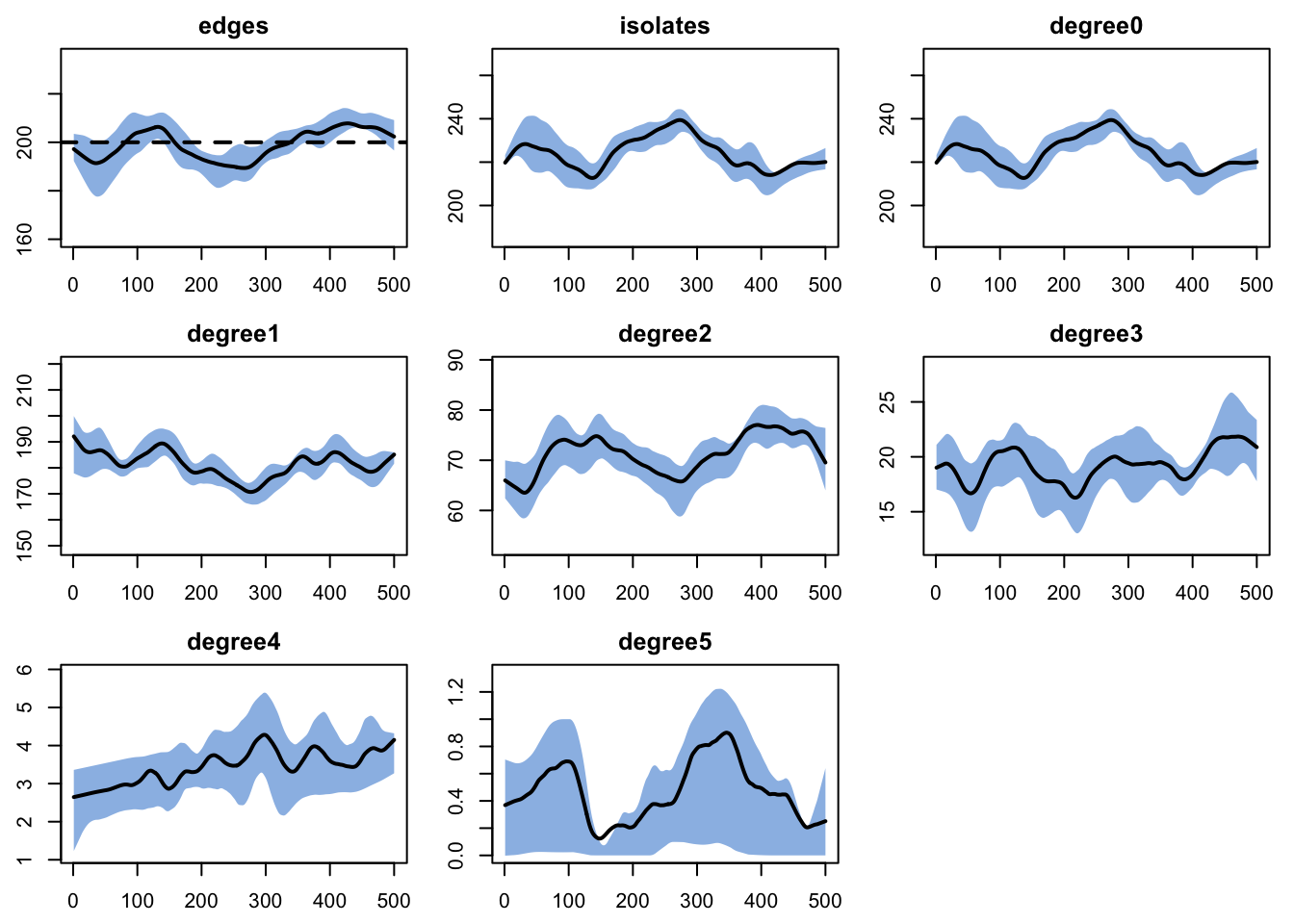

Figure 1: Network diagnostics showing edge count stability over time. The simulated mean (solid line) should track close to the target statistic (dashed line), with quantile bands capturing stochastic variation.

Epidemic Simulation

Initial Conditions

We seed the epidemic with 20 infected nodes (4% initial prevalence). All other nodes start as susceptible; the initialization module will then apply initial vaccination coverage.

init <- init.net(i.num = 20)

Control Settings

The control settings register the custom modules and specify the module execution order. Setting resimulate.network = TRUE is required because the population size changes with vital dynamics, so the network must be resimulated each timestep rather than replayed from a pre-simulated sequence.

control <- control.net(
1  type = NULL,
  nsims = nsims,
  ncores = ncores,
  nsteps = nsteps,
  initAttr.FUN = init_vaccine_attrs,
  infection.FUN = infect,
  progress.FUN = progress,
  departures.FUN = dfunc,
  arrivals.FUN = afunc,
2  resimulate.network = TRUE,
  verbose = FALSE,
  module.order = c("resim_nets.FUN", "initAttr.FUN",
                   "departures.FUN", "arrivals.FUN",
                   "infection.FUN", "progress.FUN",
3                   "prevalence.FUN")
)

1: type = NULL tells EpiModel that all disease modules are user-defined, disabling the built-in SIS/SIR models.
2: resimulate.network = TRUE resimulates the network each timestep to accommodate the changing population size from births and deaths.
3: Departures and arrivals are placed before infection so the network reflects the current population when transmission is simulated. The initAttr module runs early but only operates at the first timestep.

Scenario 1: No Vaccination (SEIR Baseline)

In the baseline scenario, all vaccination rates are set to zero. The epidemic spreads through the population limited only by natural immunity (recovery to R) and demographic turnover. New susceptible arrivals continuously enter, potentially fueling recurrent transmission waves.

param_novax <- param.net(
  inf.prob = 0.5, act.rate = 1,
  ei.rate = 0.05, ir.rate = 0.05,
  departure.rate = departure_rate,
  departure.disease.mult = 2,
  arrival.rate = 0.008,
  vaccination.rate.initialization = 0,
  protection.rate.initialization = 0,
  vaccination.rate.progression = 0,
  protection.rate.progression = 0,
  vaccination.rate.arrivals = 0,
  protection.rate.arrivals = 0
)

sim_novax <- netsim(est, param_novax, init, control)
print(sim_novax)

EpiModel Simulation
=======================
Model class: netsim

Simulation Summary
-----------------------
Model type:
No. simulations: 5
No. time steps: 500
No. NW groups: 1

Fixed Parameters
---------------------------
inf.prob = 0.5
act.rate = 1
ei.rate = 0.05
ir.rate = 0.05
departure.rate = 0.008
departure.disease.mult = 2
arrival.rate = 0.008
vaccination.rate.initialization = 0
protection.rate.initialization = 0
vaccination.rate.progression = 0
protection.rate.progression = 0
vaccination.rate.arrivals = 0
protection.rate.arrivals = 0
groups = 1

Model Functions
-----------------------
initialize.FUN 
resim_nets.FUN 
summary_nets.FUN 
infection.FUN 
departures.FUN 
arrivals.FUN 
nwupdate.FUN 
prevalence.FUN 
verbose.FUN 
initAttr.FUN 
progress.FUN 

Model Output
-----------------------
Variables: s.num i.num num d.flow a.flow vac.flow prt.flow 
vac.num prt.num se.flow e.num r.num v.num ei.flow ir.flow
Networks: sim1 ... sim5
Transmissions: sim1 ... sim5

Formation Statistics
----------------------- 
      Target Sim Mean Pct Diff Sim SE Z Score SD(Sim Means) SD(Statistic)
edges    200      200        0    Inf       0        13.838        13.838


Duration Statistics
----------------------- 
      Target Sim Mean Pct Diff Sim SE Z Score SD(Sim Means) SD(Statistic)
edges     50   119.74   139.48 15.399   4.529         3.251        40.292

Dissolution Statistics
----------------------- 
      Target Sim Mean Pct Diff Sim SE  Z Score SD(Sim Means) SD(Statistic)
edges   0.02    0.004  -79.789      0 -303.711             0         0.003

Scenario 2: Strong AON Vaccination Program

The vaccination scenario uses aggressive rates: 60% of newborns are vaccinated with an 80% protection rate (yielding 48% effective newborn protection), and 5% of unvaccinated individuals receive campaign vaccination each week (also with 80% protection). Over time, the V compartment grows, reducing the susceptible pool and creating herd immunity effects.

param_vax <- param.net(
  inf.prob = 0.5, act.rate = 1,
  ei.rate = 0.05, ir.rate = 0.05,
  departure.rate = departure_rate,
  departure.disease.mult = 2,
  arrival.rate = 0.008,
  vaccination.rate.initialization = 0.05,
  protection.rate.initialization = 0.8,
  vaccination.rate.progression = 0.05,
  protection.rate.progression = 0.8,
  vaccination.rate.arrivals = 0.6,
  protection.rate.arrivals = 0.8
)

sim_vax <- netsim(est, param_vax, init, control)
print(sim_vax)

EpiModel Simulation
=======================
Model class: netsim

Simulation Summary
-----------------------
Model type:
No. simulations: 5
No. time steps: 500
No. NW groups: 1

Fixed Parameters
---------------------------
inf.prob = 0.5
act.rate = 1
ei.rate = 0.05
ir.rate = 0.05
departure.rate = 0.008
departure.disease.mult = 2
arrival.rate = 0.008
vaccination.rate.initialization = 0.05
protection.rate.initialization = 0.8
vaccination.rate.progression = 0.05
protection.rate.progression = 0.8
vaccination.rate.arrivals = 0.6
protection.rate.arrivals = 0.8
groups = 1

Model Functions
-----------------------
initialize.FUN 
resim_nets.FUN 
summary_nets.FUN 
infection.FUN 
departures.FUN 
arrivals.FUN 
nwupdate.FUN 
prevalence.FUN 
verbose.FUN 
initAttr.FUN 
progress.FUN 

Model Output
-----------------------
Variables: s.num i.num num d.flow a.flow vac.flow prt.flow 
vac.num prt.num se.flow e.num r.num v.num ei.flow ir.flow
Networks: sim1 ... sim5
Transmissions: sim1 ... sim5

Formation Statistics
----------------------- 
      Target Sim Mean Pct Diff Sim SE Z Score SD(Sim Means) SD(Statistic)
edges    200    196.2     -1.9    Inf       0        18.767        18.767


Duration Statistics
----------------------- 
      Target Sim Mean Pct Diff Sim SE Z Score SD(Sim Means) SD(Statistic)
edges     50    119.2  138.401 15.659   4.419         3.003        40.029

Dissolution Statistics
----------------------- 
      Target Sim Mean Pct Diff Sim SE  Z Score SD(Sim Means) SD(Statistic)
edges   0.02    0.004  -79.218      0 -294.272             0         0.003

Analysis

Prevalence Comparison

We compute prevalence as the proportion of the population that is infectious and compare the two scenarios side by side. This is the headline result — vaccination dramatically reduces disease prevalence through herd immunity effects.

sim_novax <- mutate_epi(sim_novax, prev = i.num / num)
sim_vax <- mutate_epi(sim_vax, prev = i.num / num)

par(mar = c(3, 3, 2, 1), mgp = c(2, 1, 0))
plot(sim_novax, y = "prev",
     main = "Prevalence: No Vaccination vs. AON Vaccination",
     ylab = "Prevalence (I / N)", xlab = "Week",
     mean.col = "firebrick", mean.lwd = 2, mean.smooth = TRUE,
     qnts.col = "firebrick", qnts.alpha = 0.2, qnts.smooth = TRUE,
     legend = FALSE)
plot(sim_vax, y = "prev",
     mean.col = "seagreen", mean.lwd = 2, mean.smooth = TRUE,
     qnts.col = "seagreen", qnts.alpha = 0.2, qnts.smooth = TRUE,
     legend = FALSE, add = TRUE)
legend("topright",
       legend = c("No Vaccination", "Strong AON Vaccination"),
       col = c("firebrick", "seagreen"), lwd = 2, bty = "n")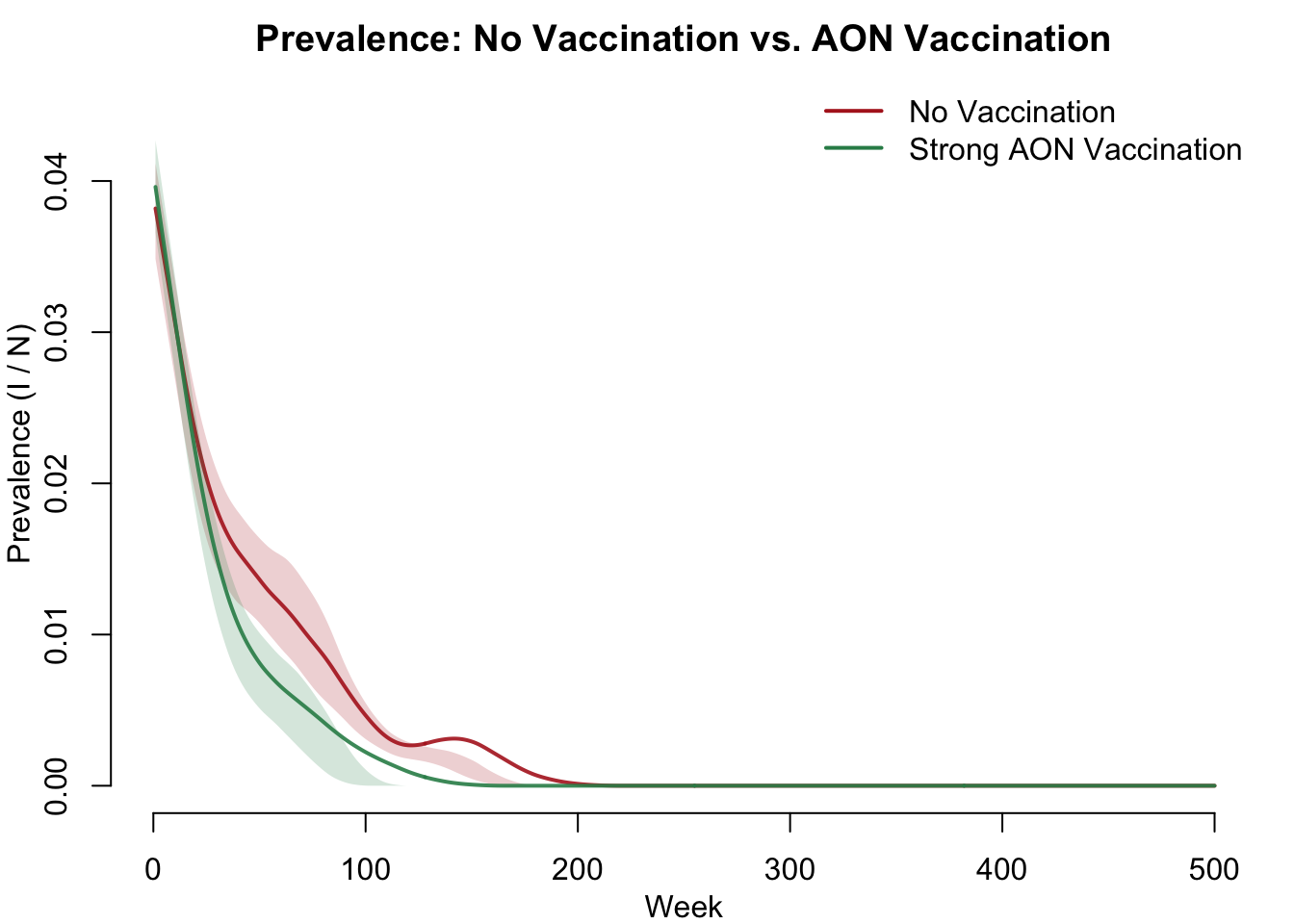

Figure 2: Prevalence comparison between the no-vaccination baseline (red) and the strong AON vaccination program (green). Solid lines show simulation means with smoothing; shaded bands show interquartile ranges across simulations.

SEIR Compartments (No Vaccination)

Without vaccination, the SEIR dynamics show the classic epidemic curve. Susceptibles decline as exposed and infectious counts rise, then recovery transfers individuals to R. Vital dynamics continuously introduce new susceptibles via births, which can fuel recurrent transmission waves.

par(mfrow = c(2, 2), mar = c(3, 3, 2, 1), mgp = c(2, 1, 0))
plot(sim_novax, y = "s.num",
     main = "Susceptible (S)", ylab = "Count", xlab = "Week",
     mean.col = "steelblue", mean.lwd = 2, mean.smooth = TRUE,
     qnts.col = "steelblue", qnts.alpha = 0.2, qnts.smooth = TRUE,
     legend = FALSE)
plot(sim_novax, y = "e.num",
     main = "Exposed (E)", ylab = "Count", xlab = "Week",
     mean.col = "#f39c12", mean.lwd = 2, mean.smooth = TRUE,
     qnts.col = "#f39c12", qnts.alpha = 0.2, qnts.smooth = TRUE,
     legend = FALSE)
plot(sim_novax, y = "i.num",
     main = "Infectious (I)", ylab = "Count", xlab = "Week",
     mean.col = "firebrick", mean.lwd = 2, mean.smooth = TRUE,
     qnts.col = "firebrick", qnts.alpha = 0.2, qnts.smooth = TRUE,
     legend = FALSE)
plot(sim_novax, y = "r.num",
     main = "Recovered (R)", ylab = "Count", xlab = "Week",
     mean.col = "seagreen", mean.lwd = 2, mean.smooth = TRUE,
     qnts.col = "seagreen", qnts.alpha = 0.2, qnts.smooth = TRUE,
     legend = FALSE)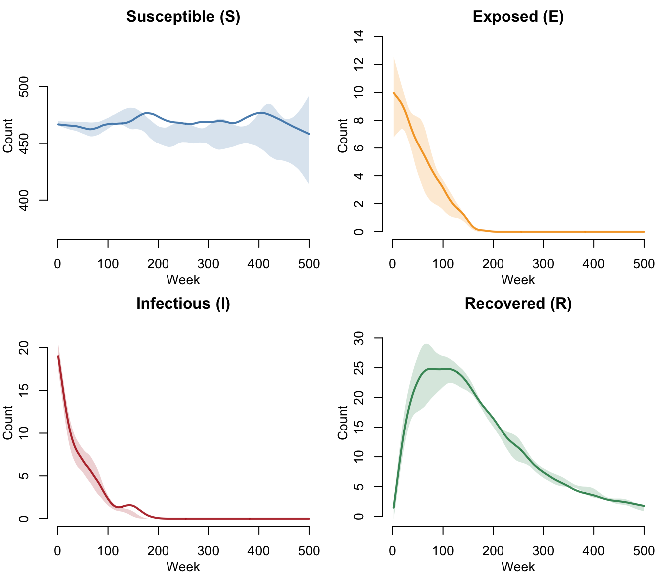

Figure 3: SEIR compartment dynamics without vaccination. New susceptible arrivals via births sustain ongoing transmission despite recovery conferring permanent natural immunity.

SEIR-V Compartments (With Vaccination)

With vaccination, the V (vaccine-immune) compartment absorbs a growing fraction of the population. This reduces the effective susceptible pool, lowering the reproductive number and suppressing the epidemic. The five-panel layout shows all compartments including the vaccine-immune class.

par(mfrow = c(2, 3), mar = c(3, 3, 2, 1), mgp = c(2, 1, 0))
plot(sim_vax, y = "s.num",
     main = "Susceptible (S)", ylab = "Count", xlab = "Week",
     mean.col = "steelblue", mean.lwd = 2, mean.smooth = TRUE,
     qnts.col = "steelblue", qnts.alpha = 0.2, qnts.smooth = TRUE,
     legend = FALSE)
plot(sim_vax, y = "e.num",
     main = "Exposed (E)", ylab = "Count", xlab = "Week",
     mean.col = "#f39c12", mean.lwd = 2, mean.smooth = TRUE,
     qnts.col = "#f39c12", qnts.alpha = 0.2, qnts.smooth = TRUE,
     legend = FALSE)
plot(sim_vax, y = "i.num",
     main = "Infectious (I)", ylab = "Count", xlab = "Week",
     mean.col = "firebrick", mean.lwd = 2, mean.smooth = TRUE,
     qnts.col = "firebrick", qnts.alpha = 0.2, qnts.smooth = TRUE,
     legend = FALSE)
plot(sim_vax, y = "r.num",
     main = "Recovered (R)", ylab = "Count", xlab = "Week",
     mean.col = "seagreen", mean.lwd = 2, mean.smooth = TRUE,
     qnts.col = "seagreen", qnts.alpha = 0.2, qnts.smooth = TRUE,
     legend = FALSE)
plot(sim_vax, y = "v.num",
     main = "Vaccine-Immune (V)", ylab = "Count", xlab = "Week",
     mean.col = "#8e44ad", mean.lwd = 2, mean.smooth = TRUE,
     qnts.col = "#8e44ad", qnts.alpha = 0.2, qnts.smooth = TRUE,
     legend = FALSE)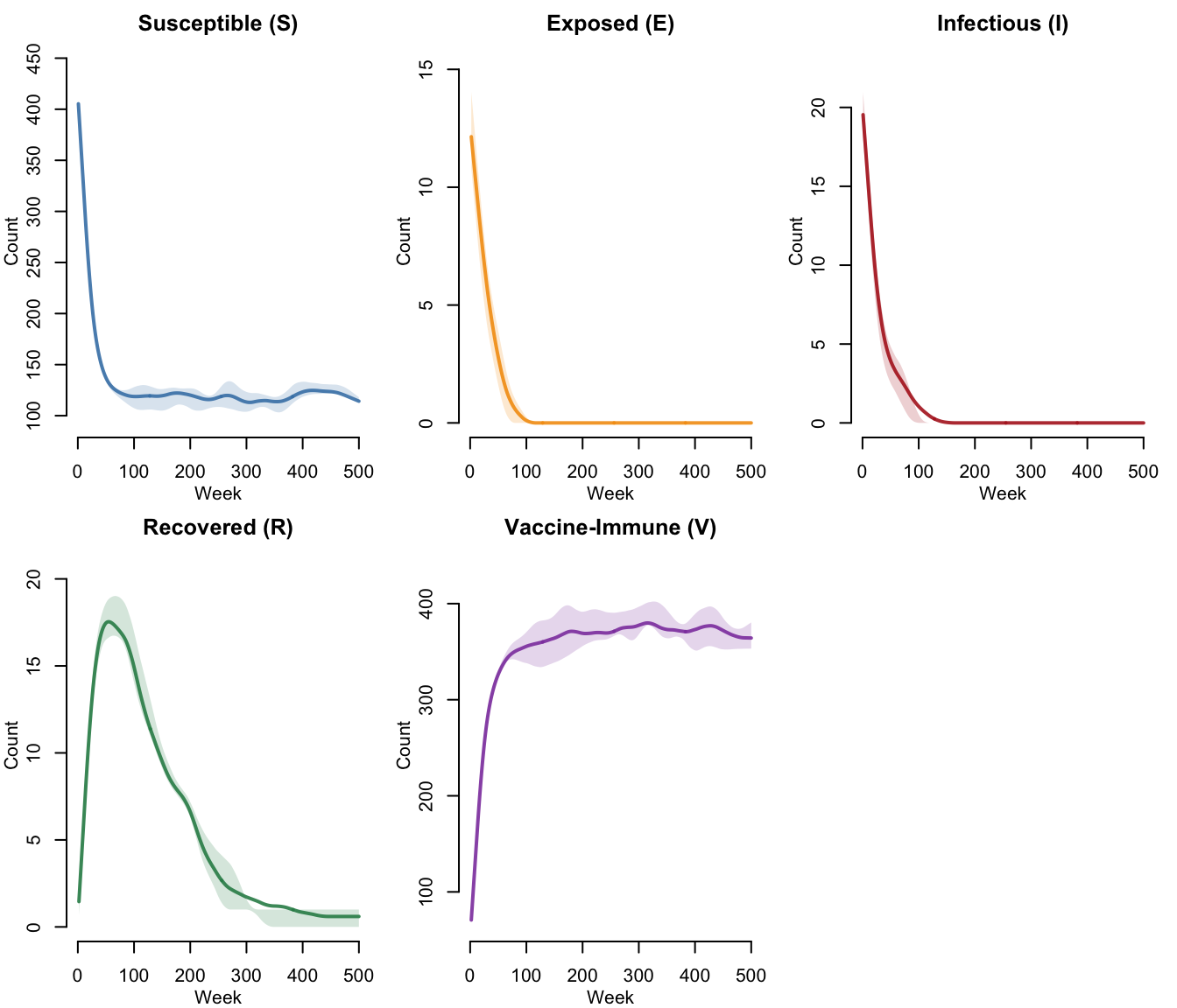

Figure 4: SEIR-V compartment dynamics with strong AON vaccination. The growing V compartment (purple) reduces the susceptible pool and suppresses the epidemic through herd immunity.

Vaccine Coverage Over Time

The vaccine-immune population grows over time as vaccination campaigns and newborn vaccination accumulate protected individuals. This plot shows the V compartment trajectory in isolation.

par(mar = c(3, 3, 2, 1), mgp = c(2, 1, 0))
plot(sim_vax, y = "v.num",
     main = "Vaccine-Immune Population Over Time",
     ylab = "Count (V)", xlab = "Week",
     mean.col = "#8e44ad", mean.lwd = 2, mean.smooth = TRUE,
     qnts.col = "#8e44ad", qnts.alpha = 0.2, qnts.smooth = TRUE,
     legend = FALSE)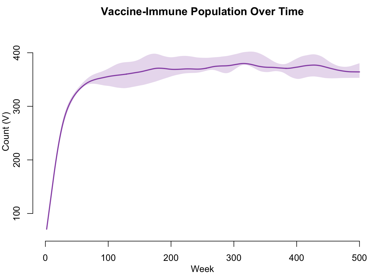

Figure 5: Growth of the vaccine-immune (V) population over time under the strong AON vaccination program. The steady accumulation of protected individuals drives the herd immunity effect.

Incidence Comparison

New infections (S-to-E transitions) per week measure the force of infection. Vaccination reduces incidence by shrinking the susceptible pool available for transmission.

par(mar = c(3, 3, 2, 1), mgp = c(2, 1, 0))
plot(sim_novax, y = "se.flow",
     main = "New Infections per Week",
     ylab = "New Infections (S -> E)", xlab = "Week",
     mean.col = "firebrick", mean.lwd = 2, mean.smooth = TRUE,
     qnts.col = "firebrick", qnts.alpha = 0.2, qnts.smooth = TRUE,
     legend = FALSE)
plot(sim_vax, y = "se.flow",
     mean.col = "seagreen", mean.lwd = 2, mean.smooth = TRUE,
     qnts.col = "seagreen", qnts.alpha = 0.2, qnts.smooth = TRUE,
     legend = FALSE, add = TRUE)
legend("topright",
       legend = c("No Vaccination", "Strong AON Vaccination"),
       col = c("firebrick", "seagreen"), lwd = 2, bty = "n")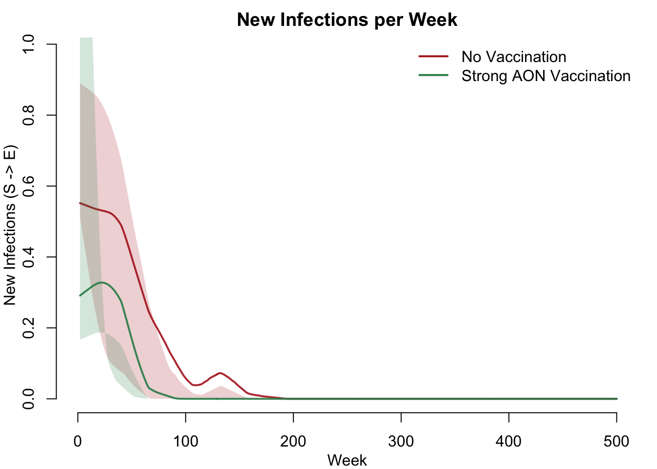

Figure 6: Weekly new infections (S to E flow) comparing the no-vaccination baseline (red) with the strong AON vaccination program (green). Vaccination reduces the incidence rate by shrinking the susceptible pool.

Summary Statistics

We extract simulation data and compute summary metrics over the final 20% of the simulation period to compare steady-state outcomes across scenarios.

df_novax <- as.data.frame(sim_novax)
df_vax <- as.data.frame(sim_vax)

late_novax <- df_novax$time > nsteps * 0.8
late_vax <- df_vax$time > nsteps * 0.8

data.frame(
  Metric = c("Mean prevalence",
             "Final prevalence",
             "Cumulative infections",
             "Mean population size",
             "Mean vaccine-immune (V)"),
  No_Vaccination = c(
    round(mean(df_novax$prev[late_novax], na.rm = TRUE), 3),
    round(mean(df_novax$prev[df_novax$time == max(df_novax$time)],
               na.rm = TRUE), 3),
    round(mean(tapply(df_novax$se.flow, df_novax$sim, sum, na.rm = TRUE))),
    round(mean(df_novax$num[late_novax], na.rm = TRUE)),
    0
  ),
  Strong_AON = c(
    round(mean(df_vax$prev[late_vax], na.rm = TRUE), 3),
    round(mean(df_vax$prev[df_vax$time == max(df_vax$time)],
               na.rm = TRUE), 3),
    round(mean(tapply(df_vax$se.flow, df_vax$sim, sum, na.rm = TRUE))),
    round(mean(df_vax$num[late_vax], na.rm = TRUE)),
    round(mean(df_vax$v.num[late_vax], na.rm = TRUE))
  )
)

                   Metric No_Vaccination Strong_AON
1         Mean prevalence              0          0
2        Final prevalence              0          0
3   Cumulative infections             44         19
4    Mean population size            471        494
5 Mean vaccine-immune (V)              0        371

Parameters

Transmission Parameters

Parameter	Description	Value
`inf.prob`	Per-act transmission probability	0.5
`act.rate`	Acts per partnership per week	1

Disease Progression Parameters

Parameter	Description	Value
`ei.rate`	E to I rate (mean latent period ~20 weeks)	0.05
`ir.rate`	I to R rate (mean infectious period ~20 weeks)	0.05

Vital Dynamics Parameters

Parameter	Description	Value
`departure.rate`	Baseline weekly mortality rate	0.008
`departure.disease.mult`	Mortality multiplier for infected	2
`arrival.rate`	Per-capita weekly birth rate	0.008

Vaccination Parameters (All-or-Nothing)

Parameter	Description	Strong Vax
`vaccination.rate.initialization`	Initial population vaccination rate	0.05
`protection.rate.initialization`	Protection rate for initial vaccinees	0.8
`vaccination.rate.progression`	Weekly campaign vaccination rate	0.05
`protection.rate.progression`	Protection rate for campaign vaccinees	0.8
`vaccination.rate.arrivals`	Newborn vaccination rate	0.6
`protection.rate.arrivals`	Protection rate for vaccinated newborns	0.8

Network Parameters

Parameter	Description	Value
Population size	Number of nodes	500
Mean degree	Average concurrent partnerships	0.8
Partnership duration	Mean edge duration (weeks)	50

Module Execution Order

The modules run in the following order at each timestep:

resim_nets -> initAttr -> departures -> arrivals -> infection -> progress -> prevalence

Departures and arrivals are placed before infection so the network reflects the current population when transmission is simulated. The initAttr module only operates at the first timestep to set up vaccination attributes. The network is resimulated first because the population size may have changed from the prior timestep’s vital dynamics.

Next Steps

Add waning vaccine immunity to convert V back to S, making vaccine protection temporary (SEIR-V with waning). This would require adding a vs.rate parameter and logic in the progression module.
Compare with leaky vaccination — see SEIRS with Leaky Vaccination for the alternative vaccine model where protection reduces but does not eliminate transmission probability.
Add booster doses by allowing re-vaccination of individuals whose protection has waned, extending the one-shot assumption to a multi-dose schedule.
Implement age-targeted vaccination by combining with age attributes — see SI with Vital Dynamics for the age module pattern.
Model vaccine hesitancy by making vaccination rates heterogeneous across individuals or network neighborhoods.
Add cost-effectiveness analysis to evaluate the vaccination program’s economic efficiency — see Cost-Effectiveness Analysis for the cost and QALY tracking framework.