SEIR/SEIRS Model: Adding an Exposed State

SEIR

SEIRS

exposed state

beginner

Extend EpiModel’s SIR by adding a latent Exposed compartment, with an SEIRS waning-immunity extension.

Author

Samuel M. Jenness

Published

August 1, 2018

Overview

Many infectious diseases have an incubation period during which a person has been infected but is not yet infectious to others. Influenza, measles, and COVID-19 all exhibit this latent stage. The standard SIR model skips it entirely — newly infected individuals become immediately infectious — but adding an Exposed (E) compartment creates an SEIR model that captures this biologically important delay between infection and infectiousness.

This example shows how to extend EpiModel’s built-in SIR framework by replacing the infection and recovery modules with two custom functions: one that routes newly infected individuals into the E compartment instead of directly to I, and a progression module that handles the E-to-I-to-R cascade. The same progression module also supports an SEIRS extension where recovered individuals eventually lose immunity and return to the susceptible pool. This single parameter change — setting rs.rate above zero — fundamentally alters the long-run dynamics, transforming an epidemic that burns out into one that persists endemically.

The techniques demonstrated here — replacing a built-in infection module, writing a custom progression module, and tracking new compartment counts — are the building blocks for all the more complex models in the Gallery.

Download standalone scripts

model.R — Main simulation script
module-fx.R — Custom module functions

Model Structure

Compartment	Label	Description
Susceptible	S	Not infected; at risk of exposure
Exposed	E	Infected but not yet infectious (latent period)
Infectious	I	Infected and capable of transmitting to contacts
Recovered	R	Immune after recovery; permanent (SEIR) or temporary (SEIRS)

flowchart LR
    S["<b>S</b><br/>Susceptible"] -->|"infection<br/>(se.flow)"| E
    E["<b>E</b><br/>Exposed"] -->|"progression<br/>(ei.flow)"| I
    I["<b>I</b><br/>Infectious"] -->|"recovery<br/>(ir.flow)"| R
    R["<b>R</b><br/>Recovered"] -.->|"waning immunity<br/>(rs.flow, SEIRS only)"| S

    style S fill:#3498db,color:#fff
    style E fill:#f39c12,color:#fff
    style I fill:#e74c3c,color:#fff
    style R fill:#27ae60,color:#fff

Transmission occurs along discordant edges — partnerships where one node is susceptible and the other is infectious. For each discordant pair, the per-timestep transmission probability accounts for multiple acts per partnership: finalProb = 1 - (1 - inf.prob) ^ act.rate. With the default parameters (inf.prob = 0.5, act.rate = 2), this gives a per-partnership probability of 0.75 per timestep.

Each transition (E to I, I to R, R to S) is modeled as an independent Bernoulli trial at each timestep: every eligible individual has a constant probability of transitioning, regardless of how long they have been in their current compartment. This produces geometrically distributed waiting times with mean 1/rate.

Setup

suppressMessages(library(EpiModel))

nsims <- 5
ncores <- 5
nsteps <- 800

Custom Modules

Infection Module

This module replaces EpiModel’s built-in infection function. The critical difference from a standard SIR infection module is that newly infected individuals enter the "e" (Exposed) state rather than becoming immediately infectious. The module extracts discordant edges via discord_edgelist(), computes per-partnership transmission probabilities accounting for multiple acts, and draws stochastic transmission events.

infect <- function(dat, at) {

  ## Attributes ##
  active <- get_attr(dat, "active")
  status <- get_attr(dat, "status")
  infTime <- get_attr(dat, "infTime")

  ## Parameters ##
  inf.prob <- get_param(dat, "inf.prob")
  act.rate <- get_param(dat, "act.rate")

  ## Find infected nodes ##
  idsInf <- which(active == 1 & status == "i")
  nActive <- sum(active == 1)
  nElig <- length(idsInf)

  ## Initialize default incidence at 0 ##
  nInf <- 0

  ## If any infected nodes, proceed with transmission ##
  if (nElig > 0 && nElig < nActive) {

    ## Look up discordant edgelist ##
1    del <- discord_edgelist(dat, at)

    ## If any discordant pairs, proceed ##
    if (!(is.null(del))) {

      # Set parameters on discordant edgelist data frame
      del$transProb <- inf.prob
      del$actRate <- act.rate
2      del$finalProb <- 1 - (1 - del$transProb)^del$actRate

      # Stochastic transmission process
3      transmit <- rbinom(nrow(del), 1, del$finalProb)

      # Keep rows where transmission occurred
      del <- del[which(transmit == 1), ]

      # Look up new ids if any transmissions occurred
      idsNewInf <- unique(del$sus)
      nInf <- length(idsNewInf)

      # Set new attributes for those newly infected
      if (nInf > 0) {
4        status[idsNewInf] <- "e"
        infTime[idsNewInf] <- at
        dat <- set_attr(dat, "status", status)
        dat <- set_attr(dat, "infTime", infTime)
      }
    }
  }

  ## Save summary statistic for S->E flow
  dat <- set_epi(dat, "se.flow", at, nInf)

  return(dat)
}

1: discord_edgelist() returns all active edges where one partner is susceptible and the other infectious.
2: Per-partnership probability: with act.rate acts, the chance of at least one successful transmission is 1 - P(all acts fail).
3: Each discordant pair independently transmits (or not) via a Bernoulli draw.
4: The key SEIR difference: newly infected individuals enter status "e" (Exposed), not "i" (Infectious).

Progression Module

This module replaces EpiModel’s built-in recovery function and handles up to three transitions: E to I, I to R, and optionally R to S. The R-to-S waning immunity block only activates when rs.rate > 0, so a single function handles both SEIR and SEIRS dynamics without code duplication.

progress <- function(dat, at) {

  ## Attributes ##
  active <- get_attr(dat, "active")
  status <- get_attr(dat, "status")

  ## Parameters ##
  ei.rate <- get_param(dat, "ei.rate")
  ir.rate <- get_param(dat, "ir.rate")
  rs.rate <- get_param(dat, "rs.rate")

  ## E to I progression process ##
  nInf <- 0
  idsEligInf <- which(active == 1 & status == "e")
  nEligInf <- length(idsEligInf)

  if (nEligInf > 0) {
1    vecInf <- which(rbinom(nEligInf, 1, ei.rate) == 1)
    if (length(vecInf) > 0) {
      idsInf <- idsEligInf[vecInf]
      nInf <- length(idsInf)
      status[idsInf] <- "i"
    }
  }

  ## I to R progression process ##
  nRec <- 0
  idsEligRec <- which(active == 1 & status == "i")
  nEligRec <- length(idsEligRec)

  if (nEligRec > 0) {
    vecRec <- which(rbinom(nEligRec, 1, ir.rate) == 1)
    if (length(vecRec) > 0) {
      idsRec <- idsEligRec[vecRec]
      nRec <- length(idsRec)
      status[idsRec] <- "r"
    }
  }

  ## R to S waning immunity process (active only when rs.rate > 0) ##
  nSus <- 0

2  if (rs.rate > 0) {
    idsEligSus <- which(active == 1 & status == "r")
    nEligSus <- length(idsEligSus)

    if (nEligSus > 0) {
      vecSus <- which(rbinom(nEligSus, 1, rs.rate) == 1)
      if (length(vecSus) > 0) {
        idsSus <- idsEligSus[vecSus]
        nSus <- length(idsSus)
        status[idsSus] <- "s"
      }
    }
  }

  ## Write out updated status attribute ##
  dat <- set_attr(dat, "status", status)

  ## Save summary statistics ##
  dat <- set_epi(dat, "ei.flow", at, nInf)
  dat <- set_epi(dat, "ir.flow", at, nRec)
  dat <- set_epi(dat, "rs.flow", at, nSus)
3  dat <- set_epi(dat, "e.num", at, sum(active == 1 & status == "e"))
  dat <- set_epi(dat, "r.num", at, sum(active == 1 & status == "r"))

  return(dat)
}

1: Each exposed individual independently transitions to infectious with probability ei.rate per timestep (Bernoulli trial), producing geometrically distributed latent durations with mean 1/ei.rate.
2: The R-to-S block is skipped entirely when rs.rate = 0, giving standard SEIR dynamics. Setting rs.rate > 0 enables the SEIRS waning-immunity extension.
3: Custom compartment counts (e.num, r.num) must be tracked manually because the built-in prevalence.net module only knows about s.num, i.num, and num.

Network Model

n <- 500
nw <- network_initialize(n)

# Formation model: edges + isolates
1formation <- ~edges + isolates
target.stats <- c(150, 240)

# Partnership duration: mean of 25 timesteps
2coef.diss <- dissolution_coefs(dissolution = ~offset(edges), duration = 25)
coef.diss

# Fit the ERGM
est <- netest(nw, formation, target.stats, coef.diss)

1: With 150 edges (mean degree = 0.6) and 240 isolates (48% of nodes with no active partnership), this produces a sparse network where roughly half the population has no current contact.
2: Closed population (no vital dynamics), so no mortality adjustment (d.rate) is needed for dissolution coefficients.

Dissolution Coefficients
=======================
Dissolution Model: ~offset(edges)
Target Statistics: 25
Crude Coefficient: 3.178054
Mortality/Exit Rate: 0
Adjusted Coefficient: 3.178054

Network Diagnostics

dx <- netdx(est, nsims = nsims, ncores = ncores, nsteps = nsteps,
            nwstats.formula = ~edges + isolates + degree(0:5))


Network Diagnostics
-----------------------
- Simulating 5 networks
- Calculating formation statistics

print(dx)

EpiModel Network Diagnostics
=======================
Diagnostic Method: Dynamic
Simulations: 5
Time Steps per Sim: 800

Formation Diagnostics
----------------------- 
         Target Sim Mean Pct Diff Sim SE Z Score SD(Sim Means) SD(Statistic)
edges       150  147.084   -1.944  0.706  -4.129         2.213         8.866
isolates    240  244.281    1.784  0.964   4.443         2.767        13.502
degree0      NA  244.281       NA  0.964      NA         2.767        13.502
degree1      NA  220.807       NA  0.819      NA         1.556        12.248
degree2      NA   31.594       NA  0.387      NA         1.422         5.714
degree3      NA    3.101       NA  0.112      NA         0.230         1.776
degree4      NA    0.212       NA  0.023      NA         0.049         0.456
degree5      NA    0.004       NA  0.002      NA         0.003         0.063

Duration Diagnostics
----------------------- 
      Target Sim Mean Pct Diff Sim SE Z Score SD(Sim Means) SD(Statistic)
edges     25   24.963   -0.148  0.185    -0.2         0.617         1.911

Dissolution Diagnostics
----------------------- 
      Target Sim Mean Pct Diff Sim SE Z Score SD(Sim Means) SD(Statistic)
edges   0.04     0.04   -0.428      0   -0.73         0.001         0.016

plot(dx)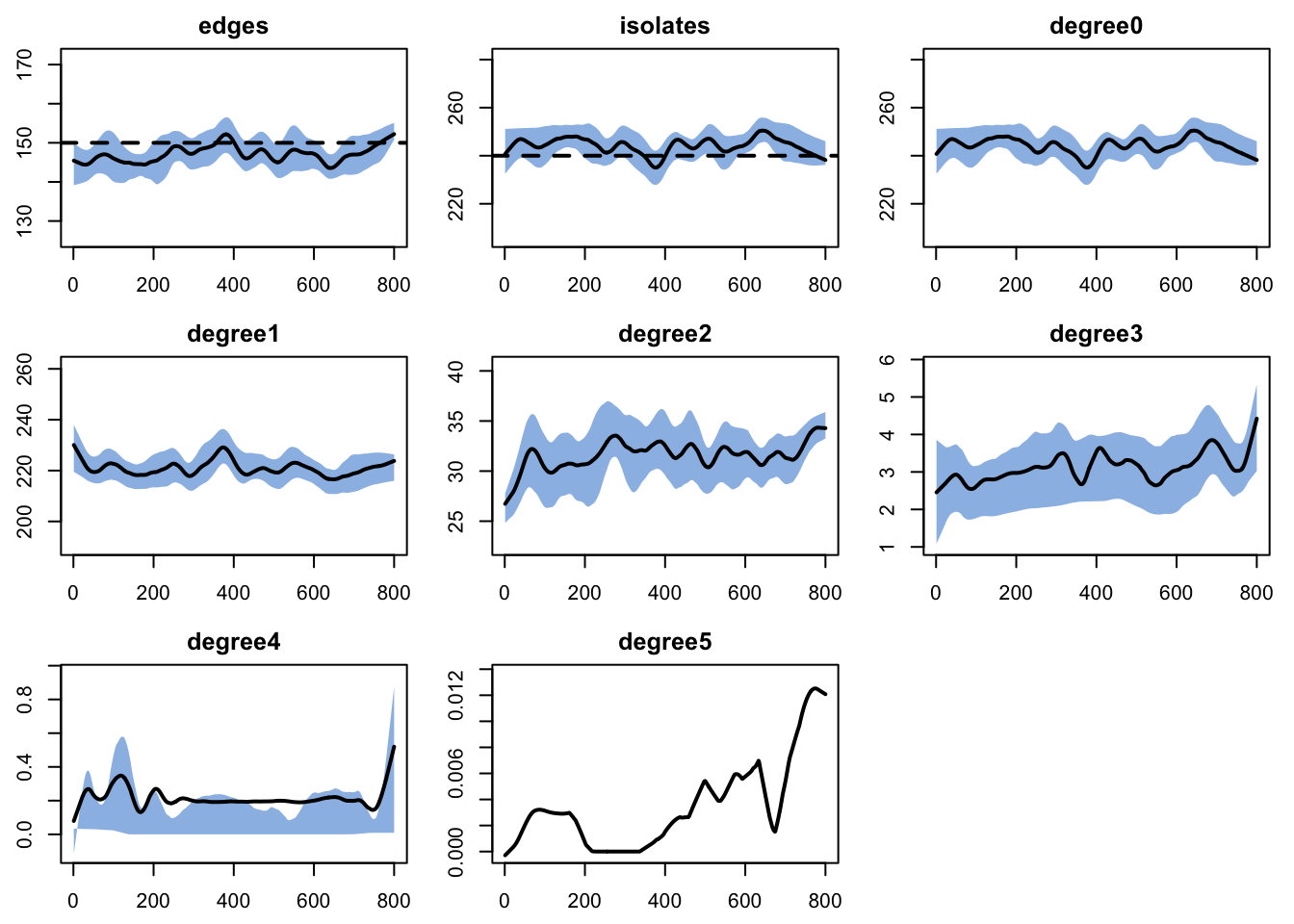

Figure 1: Network diagnostic plots verifying the simulation reproduces target statistics for edges, isolates, and degree distribution.

Epidemic Simulation

Initial Conditions

The epidemic is seeded with 10 infectious nodes (2% prevalence).

init <- init.net(i.num = 10)

Scenario 1: SEIR (Permanent Immunity)

In the SEIR model, recovered individuals gain permanent immunity (rs.rate = 0). The epidemic burns through the susceptible population and dies out once the effective reproduction number drops below 1.

param_seir <- param.net(
  inf.prob = 0.5,
  act.rate = 2,
1  ei.rate = 1 / 50,
  ir.rate = 1 / 75,
2  rs.rate = 0
)

control <- control.net(
3  type = NULL,
  nsteps = nsteps,
  nsims = nsims,
  ncores = ncores,
  infection.FUN = infect,
  progress.FUN = progress
)

sim_seir <- netsim(est, param_seir, init, control)
print(sim_seir)

1: Mean latent (E) duration of 50 timesteps; mean infectious (I) duration of 75 timesteps. These are stylized for pedagogical clarity — for influenza, typical values would be ei.rate ~ 1/2 and ir.rate ~ 1/5.
2: rs.rate = 0 means permanent immunity after recovery (standard SEIR).
3: type = NULL signals that all disease modules are custom-supplied, not built-in.

EpiModel Simulation
=======================
Model class: netsim

Simulation Summary
-----------------------
Model type:
No. simulations: 5
No. time steps: 800
No. NW groups: 1

Fixed Parameters
---------------------------
inf.prob = 0.5
act.rate = 2
ei.rate = 0.02
ir.rate = 0.01333333
rs.rate = 0
groups = 1

Model Functions
-----------------------
initialize.FUN 
resim_nets.FUN 
summary_nets.FUN 
infection.FUN 
nwupdate.FUN 
prevalence.FUN 
verbose.FUN 
progress.FUN 

Model Output
-----------------------
Variables: s.num i.num num ei.flow ir.flow rs.flow e.num 
r.num se.flow
Networks: sim1 ... sim5
Transmissions: sim1 ... sim5

Formation Statistics
----------------------- 
         Target Sim Mean Pct Diff Sim SE Z Score SD(Sim Means) SD(Statistic)
edges       150  147.382   -1.745  0.674  -3.885         1.746         9.043
isolates    240  244.291    1.788  1.025   4.188         2.430        13.906


Duration Statistics
----------------------- 
      Target Sim Mean Pct Diff Sim SE Z Score SD(Sim Means) SD(Statistic)
edges     25   25.016    0.065  0.223   0.073          0.52         2.119

Dissolution Statistics
----------------------- 
      Target Sim Mean Pct Diff Sim SE Z Score SD(Sim Means) SD(Statistic)
edges   0.04     0.04    1.031      0   1.585         0.001         0.016

Scenario 2: SEIRS (Waning Immunity)

Adding waning immunity (rs.rate = 1/100) fundamentally changes the long-run dynamics. Instead of epidemic burnout, the disease persists indefinitely as recovered individuals return to the susceptible pool, creating sustained endemic transmission with periodic fluctuations.

param_seirs <- param.net(
  inf.prob = 0.5,
  act.rate = 2,
  ei.rate = 1 / 50,
  ir.rate = 1 / 75,
1  rs.rate = 1 / 100
)

sim_seirs <- netsim(est, param_seirs, init, control)
print(sim_seirs)

1: Mean immune duration of 100 timesteps before returning to S. This single change transforms the dynamics from epidemic burnout to endemic persistence.

EpiModel Simulation
=======================
Model class: netsim

Simulation Summary
-----------------------
Model type:
No. simulations: 5
No. time steps: 800
No. NW groups: 1

Fixed Parameters
---------------------------
inf.prob = 0.5
act.rate = 2
ei.rate = 0.02
ir.rate = 0.01333333
rs.rate = 0.01
groups = 1

Model Functions
-----------------------
initialize.FUN 
resim_nets.FUN 
summary_nets.FUN 
infection.FUN 
nwupdate.FUN 
prevalence.FUN 
verbose.FUN 
progress.FUN 

Model Output
-----------------------
Variables: s.num i.num num ei.flow ir.flow rs.flow e.num 
r.num se.flow
Networks: sim1 ... sim5
Transmissions: sim1 ... sim5

Formation Statistics
----------------------- 
         Target Sim Mean Pct Diff Sim SE Z Score SD(Sim Means) SD(Statistic)
edges       150  146.974   -2.017  0.752  -4.025         1.817         9.231
isolates    240  244.928    2.053  0.959   5.138         2.162        13.341


Duration Statistics
----------------------- 
      Target Sim Mean Pct Diff Sim SE Z Score SD(Sim Means) SD(Statistic)
edges     25   24.802   -0.791    0.2  -0.987         0.445         1.933

Dissolution Statistics
----------------------- 
      Target Sim Mean Pct Diff Sim SE Z Score SD(Sim Means) SD(Statistic)
edges   0.04     0.04    1.116      0   1.709             0         0.017

Analysis

sim_seir <- mutate_epi(sim_seir, prev = i.num / num)
sim_seirs <- mutate_epi(sim_seirs, prev = i.num / num)

Prevalence Comparison

The central question: how does waning immunity change disease burden? In the SEIR model, prevalence rises then falls to zero as immunity accumulates and susceptibles are exhausted. In the SEIRS model, prevalence stabilizes at an endemic level because recovered individuals continuously return to the susceptible pool.

par(mfrow = c(1, 1), mar = c(3, 3, 2, 1), mgp = c(2, 1, 0))
plot(sim_seir, y = "prev",
     main = "Prevalence: SEIR vs. SEIRS",
     ylab = "Prevalence (I / N)", xlab = "Time Step",
     mean.col = "firebrick", mean.lwd = 2, mean.smooth = TRUE,
     qnts.col = "firebrick", qnts.alpha = 0.2, qnts.smooth = TRUE,
     legend = FALSE)
plot(sim_seirs, y = "prev",
     mean.col = "steelblue", mean.lwd = 2, mean.smooth = TRUE,
     qnts.col = "steelblue", qnts.alpha = 0.2, qnts.smooth = TRUE,
     legend = FALSE, add = TRUE)
legend("topright", legend = c("SEIR", "SEIRS"),
       col = c("firebrick", "steelblue"), lwd = 2, bty = "n")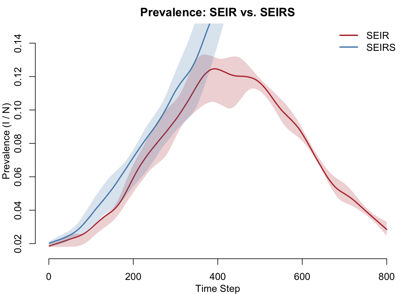

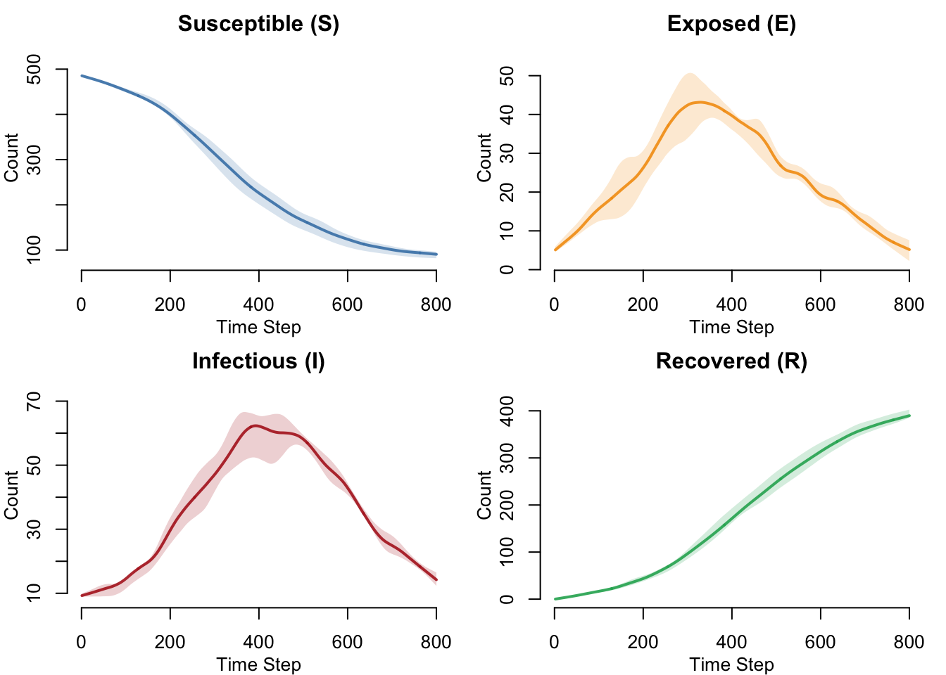
Figure 2: Prevalence over time. Red: SEIR with permanent immunity (epidemic burnout). Blue: SEIRS with waning immunity (endemic persistence).

SEIR Compartment Dynamics

All four compartments over time in the standard SEIR model. The classic SEIR trajectory shows S declining as individuals are infected, E and I rising then falling as the epidemic wave passes, and R accumulating toward the full population as immunity builds.

compartments <- c("s.num", "e.num", "i.num", "r.num")
titles <- c("Susceptible (S)", "Exposed (E)", "Infectious (I)", "Recovered (R)")
colors <- c("steelblue", "#f39c12", "firebrick", "#27ae60")

par(mfrow = c(2, 2), mar = c(3, 3, 2, 1), mgp = c(2, 1, 0))
for (j in seq_along(compartments)) {
  plot(sim_seir, y = compartments[j],
       main = titles[j], ylab = "Count", xlab = "Time Step",
       mean.col = colors[j], mean.lwd = 2, mean.smooth = TRUE,
       qnts.col = colors[j], qnts.alpha = 0.2, qnts.smooth = TRUE,
       legend = FALSE)
}

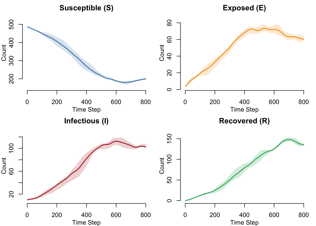
Figure 3: SEIR compartment dynamics. S declines, E and I rise and fall with the epidemic wave, and R accumulates toward the full population.

SEIRS Compartment Dynamics

With waning immunity, S does not deplete permanently and R does not accumulate forever. The system reaches a dynamic equilibrium with all four compartments maintaining nonzero populations — a hallmark of endemic disease dynamics.

par(mfrow = c(2, 2), mar = c(3, 3, 2, 1), mgp = c(2, 1, 0))
for (j in seq_along(compartments)) {
  plot(sim_seirs, y = compartments[j],
       main = titles[j], ylab = "Count", xlab = "Time Step",
       mean.col = colors[j], mean.lwd = 2, mean.smooth = TRUE,
       qnts.col = colors[j], qnts.alpha = 0.2, qnts.smooth = TRUE,
       legend = FALSE)
}

Figure 4: SEIRS compartment dynamics. With waning immunity, the system reaches dynamic equilibrium rather than epidemic burnout.

New Infections (Incidence)

In the SEIR model, incidence peaks then declines to zero as susceptibles are exhausted. In the SEIRS model, incidence is sustained by the continuous resupply of susceptibles from recovered individuals losing immunity.

par(mfrow = c(1, 1), mar = c(3, 3, 2, 1), mgp = c(2, 1, 0))
plot(sim_seir, y = "se.flow",
     main = "New Infections: SEIR vs. SEIRS",
     ylab = "New Infections per Timestep", xlab = "Time Step",
     mean.col = "firebrick", mean.lwd = 2, mean.smooth = TRUE,
     qnts.col = "firebrick", qnts.alpha = 0.2, qnts.smooth = TRUE,
     legend = FALSE)
plot(sim_seirs, y = "se.flow",
     mean.col = "steelblue", mean.lwd = 2, mean.smooth = TRUE,
     qnts.col = "steelblue", qnts.alpha = 0.2, qnts.smooth = TRUE,
     legend = FALSE, add = TRUE)
legend("topright", legend = c("SEIR", "SEIRS"),
       col = c("firebrick", "steelblue"), lwd = 2, bty = "n")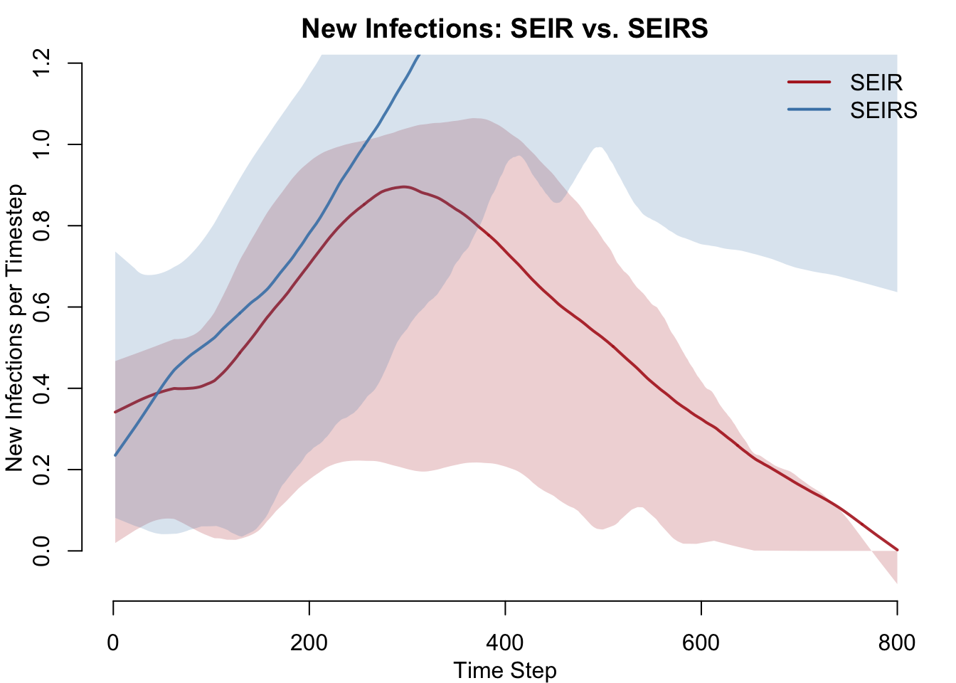

Figure 5: New infections per timestep. SEIR incidence declines to zero; SEIRS incidence is sustained by the continuous resupply of susceptibles.

Summary Table

df_seir <- as.data.frame(sim_seir)
df_seirs <- as.data.frame(sim_seirs)

knitr::kable(data.frame(
  Metric = c("Peak prevalence",
             "Mean prevalence",
             "Cumulative infections",
             "Final recovered count"),
  SEIR = c(
    round(max(tapply(df_seir$prev, df_seir$sim, max, na.rm = TRUE)), 3),
    round(mean(df_seir$prev, na.rm = TRUE), 3),
    round(mean(tapply(df_seir$se.flow, df_seir$sim, sum, na.rm = TRUE))),
    round(mean(df_seir$r.num[df_seir$time == max(df_seir$time)], na.rm = TRUE))
  ),
  SEIRS = c(
    round(max(tapply(df_seirs$prev, df_seirs$sim, max, na.rm = TRUE)), 3),
    round(mean(df_seirs$prev, na.rm = TRUE), 3),
    round(mean(tapply(df_seirs$se.flow, df_seirs$sim, sum, na.rm = TRUE))),
    round(mean(df_seirs$r.num[df_seirs$time == max(df_seirs$time)], na.rm = TRUE))
  )
))

Table 1

Metric	SEIR	SEIRS
Peak prevalence	0.180	0.264
Mean prevalence	0.073	0.142
Cumulative infections	400.000	918.000
Final recovered count	390.000	137.000

Parameters

Transmission

Parameter	Description	Default
`inf.prob`	Per-act transmission probability	0.5
`act.rate`	Acts per partnership per timestep	2

Disease Progression

Parameter	Description	Default
`ei.rate`	E-to-I rate (1 / mean latent duration)	1/50
`ir.rate`	I-to-R rate (1 / mean infectious duration)	1/75
`rs.rate`	R-to-S waning immunity rate (0 = permanent immunity)	0 (SEIR) or 1/100 (SEIRS)

Network

Parameter	Description	Default
Population size	Number of nodes	500
Target edges	Mean concurrent partnerships	150
Target isolates	Nodes with degree 0	240
Partnership duration	Mean edge duration (timesteps)	25

Note

These parameters are stylized for pedagogical clarity, not calibrated to a specific pathogen. For influenza, typical values would be ei.rate ~ 1/2 and ir.rate ~ 1/5.

Module Execution Order

resim_nets → infection (infect) → progress → prevalence

The built-in prevalence.net module runs last and computes s.num, i.num, and num from the updated status attribute. The custom progress module additionally tracks e.num, r.num, and all transition flows (ei.flow, ir.flow, rs.flow).

Next Steps

Add vital dynamics (births and deaths) to maintain population size over long runs and allow true endemic equilibrium — see SI with Vital Dynamics
Incorporate vaccination using all-or-nothing or leaky mechanisms — see SEIR with AON Vaccination and SEIRS with Leaky Vaccination
Vary progression rates by individual attributes (e.g., age, immune status) to model heterogeneous disease courses
Add stage-dependent infectiousness where transmission probability depends on disease stage — see the HIV model for this pattern
Calibrate to a specific pathogen by substituting published estimates for latent and infectious period durations