flowchart LR
    S["<b>S</b>"] -->|"infection"| E
    E["<b>E</b>"] -->|"~3 days, 70%"| Ip
    E -->|"~3 days, 30%"| Ia["<b>I_a</b><br/>asymp"]
    Ip["<b>I_p</b><br/>presymp"] -->|"~2.5 days"| Is["<b>I_s</b><br/>symp"]
    Is -->|"~6 days"| R["<b>R</b>"]
    Ia -->|"~8 days"| R
    Is -.->|"diagnosis"| Q["isolate index,<br/>trace and quarantine<br/>contacts"]

    style S fill:#3498db,color:#fff
    style E fill:#9b59b6,color:#fff
    style Ip fill:#f39c12,color:#fff
    style Is fill:#e74c3c,color:#fff
    style Ia fill:#e67e22,color:#fff
    style R fill:#27ae60,color:#fff
    style Q fill:#5b3a8c,color:#fff
SEIR with Contact Tracing for an Acute, Immunizing Infection
SEIR
contact tracing
intervention
cumulative edgelist
intermediate
Contact tracing as a network intervention. A COVID-like SEIR with presymptomatic and asymptomatic transmission, symptom-based diagnosis with isolation, and a tracing module that finds each index’s recent contacts through EpiModel’s cumulative edgelist and quarantines them. Reports infections averted with Monte Carlo intervals, the state of contacts when reached, and quarantine days per infection averted.
Overview
Contact tracing is a partner-services intervention: when a person is diagnosed, public health staff elicit the people that person was in close contact with while infectious and ask them to quarantine. It is a network operation in the literal sense. The contacts that matter are the contacts the index case actually had, over a window that runs back to before the index felt ill, and some of those contacts are people the index no longer sees. A compartmental model can only represent this as an average rate. A network model with a record of past partnerships can represent it as what it is.
EpiModel keeps that record as the cumulative edgelist: a running history of every partnership the simulation has seen, with the step on which each began and ended. The get_partners() function walks the history for any set of index nodes, and a custom module can then decide what to do with the partners it returns. This example uses that machinery to build a contact tracing program for a COVID-like acute infection and to ask the questions that were asked of tracing programs in 2020:
- How much does tracing add to case isolation? Symptom-based diagnosis with isolation is the standard of care that tracing builds on. It is weak against this pathogen because about 45% of transmission from symptomatic infections happens before symptoms, and 30% of infections never produce symptoms at all (the mechanism formalized by Fraser et al. 2004). Tracing reaches the people those transmissions went to.
- Speed or coverage? The scenarios cross the delay from diagnosis to reaching contacts (1 day against 4) with the share of contacts reached (80% against 30%), the two levers of the published tracing models (Kretzschmar et al. 2020, Hellewell et al. 2020).
- What does it cost? Every reached contact is quarantined for ten days whether or not they turn out to be infected. The model reports the state each contact was in when reached (susceptible, latent, infectious, or already recovered), the number of quarantine person-days per infection averted, and the share of the population in quarantine at the peak. These are outputs that only an individual-level model can produce, and the last one is the burden that Firth et al. 2020 found dominates on a real-world network.
Every transmission is recorded with the infector’s disease stage and restriction status, so the page also checks the natural history against the literature: the share of transmission that is presymptomatic, the reproduction number, and the generation time are read from the simulation rather than asserted.
NoteHow this relates to the partner notification example and to published tracing models
The Partner Notification example uses the same cumulative-edgelist functions for an endemic sexually transmitted infection, where the intervention is treatment of notified partners and the lookback is measured in months. This example is the acute-outbreak counterpart: the pathogen is respiratory, contacts are elicited over a window of days that is anchored to symptom onset, the intervention is quarantine of contacts who are not known to be infected, and the race between tracing and the presymptomatic window is what decides the outcome. The two pages teach the same API in the two settings where it is used.
The COVID-19 tracing literature is mostly branching-process and compartmental models of a single index case and its contacts (Hellewell 2020, Kretzschmar 2020, Kucharski 2020), which report the reduction in the reproduction number that a program achieves per index. This example runs the program on a whole population over an epidemic, so it reports final sizes, quarantine burden, and the state of the contacts found, and it shows a population-level effect those models do not contain. Its parameters are illustrative, not calibrated to any outbreak.
TipDownload and run the standalone scripts
- model.R: main simulation script
- module-fx.R: custom module functions
model.R sources module-fx.R from examples/seir-contact-tracing/ when run from the repository root and from the working directory otherwise, so the two downloaded files can sit in one folder. Sourcing the script interactively (for example in RStudio) uses the full settings on this page (N = 5000, ten simulations, 250 days, two to three minutes on five cores). Rscript is not interactive and uses the small continuous-integration settings (N = 1000, one simulation, 50 days, under a minute) whose results are not meant to be interpreted; to get the full settings from the command line, pass R code that defines run_full as the first argument:
Rscript model.R "run_full <- TRUE"Model Structure
Disease Compartments
| Status | Substage | Description |
|---|---|---|
| S | Susceptible | |
| E | Exposed, latent (mean 3 days) | |
| I | inf.stage = "ip" |
Presymptomatic infectious (mean 2.5 days), for the 70% of infections that will become symptomatic |
| I | inf.stage = "is" |
Symptomatic infectious (mean 6 days), at half the per-contact infectiousness of the presymptomatic stage |
| I | inf.stage = "ia" |
Asymptomatic infectious (mean 8 days), at 35% of the presymptomatic infectiousness; these infections skip the presymptomatic stage and are never diagnosed by symptoms |
| R | Recovered, immune |
The standard status attribute holds the SEIR compartment and a separate inf.stage attribute carries the substage, so EpiModel’s built-in prevalence module, discord_edgelist(), and the standard plots all work unchanged. Every stage duration is geometric with the stated mean, because each transition is a daily Bernoulli draw.
Interventions
Two case-based interventions act through the same channel, a reduction in the daily probability of transmission across an edge:
- Diagnosis and isolation. At symptom onset, a case will seek a test with probability
dx.prob, and if so is diagnosed after a delay with meandx.delaydays. A diagnosed index isolates for the nextiso.durationdays, during which the transmission probability across its edges is multiplied byiso.mult. - Contact tracing and quarantine.
trace.delaydays after an index’s diagnosis, the tracing module finds the index’s partners whose partnership overlapped the contact elicitation window (fromtrace.windowdays before the index’s symptom onset to the day of diagnosis), reaches each one with probabilitytrace.reach.prob, and quarantines the reached contacts forquar.durationdays. While a contact is quarantined, the transmission probability across all of its edges, in both directions, is multiplied byquar.mult: a quarantined contact who is infected transmits less, and a quarantined contact who is susceptible is exposed less.
A contact who develops symptoms during quarantine can be diagnosed like any other case and then becomes an index in turn, so tracing propagates along transmission chains without any extra code.
Node attributes
| Attribute | Set by | Meaning |
|---|---|---|
inf.stage |
init_attrs, progress |
"ip", "is", or "ia" while in I; NA otherwise |
symp.time |
progress |
step of symptom onset; anchors the elicitation window |
dx.due |
progress |
step on which the case will be diagnosed (NA if it never seeks a test) |
dx.time |
progress |
step of diagnosis; at - dx.time == trace.delay triggers the trace |
iso.until |
progress |
last step of the index’s isolation |
quar.until |
trace |
last step of a contact’s quarantine |
Setup
suppressMessages(library(EpiModel))

# These are the full settings of the standalone model.R. The population is
# larger than in most Gallery examples so that the contacts found by tracing
# number in the thousands per simulation and the between-simulation noise
# is small next to the scenario differences.
N <- 5000
nsims <- 10
ncores <- 5
nsteps <- 250
# The custom modules (init_attrs, infect, progress, trace) used in
# control.net(). The excerpts under "Custom Modules" are pulled from this file.
source("module-fx.R")Network Model
A single dynamic network of close contacts, with a mean degree of 6 and a mean partnership duration of 7 days. Each time step is one day. The network is deliberately simple so that the tracing mechanism stays in focus, but its two parameters set the terms of the tracing problem. Over an infectious period of about 8 days a case has roughly 12 distinct close contacts, and by the time a tracer looks for them, about half of the partnerships in the elicitation window have already ended. Those ended partnerships are exactly what the cumulative edgelist exists to recover; a module that only read the current network would miss them.
set.seed(2026)
mean_degree <- 6
duration <- 7

nw <- network_initialize(N)
formation <- ~edges
target.stats <- round(mean_degree * N / 2)
coef.diss <- dissolution_coefs(~offset(edges), duration = duration)
est <- netest(nw, formation, target.stats, coef.diss, verbose = FALSE)

dx <- netdx(est, nsims = 5, ncores = ncores, nsteps = nsteps,
            nwstats.formula = ~edges + degree(0:4, by = NULL) + meandeg,
            verbose = FALSE)
print(dx)
EpiModel Network Diagnostics
=======================
Diagnostic Method: Dynamic
Simulations: 5
Time Steps per Sim: 250
Formation Diagnostics
-----------------------
Target Sim Mean Pct Diff Sim SE Z Score SD(Sim Means) SD(Statistic)
edges 15000 14988.066 -0.08 10.416 -1.146 14.043 116.291
degree0 NA 12.487 NA 0.170 NA 0.531 3.805
degree1 NA 74.940 NA 0.530 NA 1.000 10.237
degree2 NA 224.585 NA 0.869 NA 2.529 17.141
degree3 NA 447.873 NA 1.267 NA 1.468 22.781
degree4 NA 671.338 NA 1.129 NA 1.647 24.447
meandeg NA 5.995 NA 0.004 NA 0.006 0.047
Duration Diagnostics
-----------------------
Target Sim Mean Pct Diff Sim SE Z Score SD(Sim Means) SD(Statistic)
edges 7 7.026 0.372 0.005 5.219 0.01 0.055
Dissolution Diagnostics
-----------------------
Target Sim Mean Pct Diff Sim SE Z Score SD(Sim Means) SD(Statistic)
edges 0.143 0.142 -0.331 0 -6.05 0 0.003plot(dx)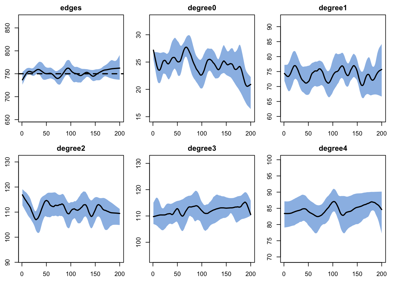
Custom Modules
Four custom modules: init_attrs (one-shot setup of the substage and intervention attributes), infect (S to E with the isolation and quarantine multipliers, recording every transmission), progress (E to Ip to Is to R or E to Ia to R, with diagnosis scheduled at symptom onset), and trace (the headline module). Full code is in module-fx.R; the parts that carry the logic are below.
trace: the cumulative-edgelist pattern
The tracing module is a five-step pattern, and the middle three steps are the EpiModel API this example exists to teach.
# 1. Indices whose trace is due today
idsIndex <- which(active == 1 & !is.na(dx.time) &
1                  (at - dx.time) == trace.delay)

if (length(idsIndex) > 0) {
  # 2. Their partners from the cumulative edgelist
2  part_df <- get_partners(dat, idsIndex, only.active.nodes = TRUE)

  if (!is.null(part_df) && nrow(part_df) > 0) {
    # 3. Keep the partnerships that overlap each index's elicitation window
    index_pid <- get_posit_ids(dat, part_df$index)
    window_start <- symp.time[index_pid] - trace.window
    window_end <- dx.time[index_pid]
    in_window <- (is.na(part_df$stop) | part_df$stop >= window_start) &
3                 part_df$start <= window_end
    part_df <- part_df[in_window, , drop = FALSE]

    # 4. Partner unique ids back to positional ids, one row per partner,
    #    dropping partners who are already diagnosed
4    partner_pid <- get_posit_ids(dat, part_df$partner)
    ended <- !is.na(part_df$stop)
    keep <- !duplicated(partner_pid) & is.na(dx.time[partner_pid])
    partner_pid <- partner_pid[keep]
    ended <- ended[keep]
    n_part <- length(partner_pid)
    n_part_ended <- sum(ended)

    if (n_part > 0) {
      # 5. Reach and quarantine
      reached <- partner_pid[rbinom(n_part, 1, trace.reach.prob) == 1]
      n_reach <- length(reached)
      if (n_reach > 0) {
        state <- ifelse(status[reached] == "i", inf.stage[reached],
5                        status[reached])
        reach_state[] <- as.numeric(table(factor(state,
                                                 levels = names(reach_state))))
        in_quar <- !is.na(quar.until[reached]) & at <= quar.until[reached]
        n_quar_start <- sum(!in_quar)
        quar.until[reached] <- pmax(quar.until[reached],
6                                    at + quar.duration, na.rm = TRUE)
      }
    }
  }
}- 1
-
Delay without a queue. An index diagnosed on step T is traced on step T +
trace.delay. Conditioning on equality rather than>=makes each index fire exactly once. - 2
-
The cumulative-edgelist call.
get_partners()takes positional ids (the indices you have in hand) and returns one row per partnership:indexandpartneras unique ids, and the partnership’sstartandstopsteps.stopis the last step on which the partnership was active and isNAwhile it is still active;start = 0marks a partnership that already existed when the simulation began. Notruncateargument is passed here because the window is applied per index in the next step;truncate = Kwould instead keep every active partnership plus those last active within the past K steps, which is the right tool when the lookback is the same for every index.only.active.nodes = TRUEdrops partners who have left the population, a no-op in this closed population but the correct call in a model with departures, where the lookup in step 4 would otherwise returnNAwith a warning. - 3
-
The elicitation window, from the returned columns. Public health guidance elicits contacts from two days before symptom onset (CDC) until the case isolated. Each row’s
startandstopare compared with that window for its own index, so an index diagnosed late in its illness reaches further back than one diagnosed early. BecausestopisNAfor active partnerships, they always qualify. - 4
-
The id round trip.
part_df$partneris in the unique-id space because a partner may have left the simulation since the partnership existed;get_posit_ids()translates back before indexing any attribute vector. In a closed population the two id spaces coincide, and the translation is still the right habit, because the moment a model adds departures it becomes load-bearing. Theendedflag records whether each partner was found through a partnership that had already dissolved, which is the share of the program’s reach that the cumulative edgelist alone can provide. - 5
- The yield. Before quarantining, the module records the state each reached contact is in: susceptible, latent, infectious (any substage), or recovered. Nothing in the tracing logic uses this; it exists so the analysis can report what a tracing program actually finds.
- 6
- Extend, never shorten. A contact who is reached again while already quarantined keeps the later of the two end dates.
infect: one multiplier for both interventions, and a transmission record
isolated <- !is.na(iso.until) & at <= iso.until
quarantined <- !is.na(quar.until) & at <= quar.until

del <- discord_edgelist(dat, at, network = 1, infstat = "i")
# ...
stage <- inf.stage[del$inf]
p <- inf.prob * ifelse(stage == "is", is.inf.mult,
1                       ifelse(stage == "ia", ia.inf.mult, 1))
restrict <- ifelse(isolated[del$inf], iso.mult, 1)
restrict <- pmin(restrict,
                 ifelse(quarantined[del$inf] | quarantined[del$sus],
2                        quar.mult, 1))
p <- p * restrict
hit <- which(rbinom(length(p), 1, p) == 1)
# ...
del$infStage <- inf.stage[del$inf]
del$infIsolated <- as.integer(isolated[del$inf])
del$anyQuarantined <- as.integer(quarantined[del$inf] | quarantined[del$sus])
del$infTime <- infTime[del$inf]
3dat <- set_transmat(dat, del, at)- 1
- Infectiousness by substage. The presymptomatic stage carries the full per-contact probability, the symptomatic stage half of it, and asymptomatic infections about a third. With the stage durations, about 45% of the transmission from symptomatic infections occurs before onset; the analysis checks this from the transmission record.
- 2
- The single line both interventions act through. Isolation applies to the infector’s edges; quarantine applies to every edge of a quarantined person, so it protects a susceptible contact as well as containing an infected one. When both apply, the stronger reduction wins.
- 3
-
Transmission record.
set_transmat()stores the rows for this step andget_transmat()returns them per simulation with the extra columns intact, which is what the source-of-transmission table, the reproduction number, and the generation time below are built from.
progress: diagnosis scheduled at symptom onset
Whether a symptomatic case will ever be diagnosed and how long that takes are separate quantities in the literature (ascertainment and testing delay), so they are separate parameters here. At the Ip to Is transition a case draws whether it will seek a test, and if so, the day of its diagnosis:
- 1
-
One plus a geometric draw gives a delay of at least one day with mean
dx.delaydays. - 2
- A case that has already recovered by its scheduled day is still diagnosed, because a test detects infection rather than infectiousness. Its isolation changes nothing, but it triggers a trace of its contacts, some of whom may still be latent.
Module order
EpiModel’s default order runs user-supplied modules before the built-in ones, which would run progress and trace ahead of infect and, more importantly, ahead of resim_nets, where the cumulative edgelist is updated. The order is set explicitly in control.net() so that each step runs
resim_nets -> summary_nets -> initAttr -> infection -> progress -> trace -> nwupdate -> prevalenceWith this order the cumulative edgelist is current when trace reads it, the day’s diagnoses are stamped before trace looks for indices whose delay has elapsed (so trace.delay = 0 would trace on the day of diagnosis), and progress requires infTime < at for the E to I transition so that a node infected this step spends at least one step in E. A module left out of module.order is skipped, with a warning from control.net() only if it is resim_nets, summary_nets, or nwupdate, and initialize.FUN and verbose.FUN are not listed because they run outside the step loop.
Parameters
Natural history. The values describe an ancestral-lineage SARS-CoV-2-like virus, with every duration geometric. A mean latent period of 3 days plus a mean presymptomatic infectious period of 2.5 days gives a mean incubation period of 5.5 days (Lauer et al. 2020; McAloon et al. 2020). The symptomatic infectious period is 6 days, within the window over which infectious virus is recovered after onset (van Kampen et al. 2021; Cevik et al. 2021), at half the per-contact infectiousness of the presymptomatic stage because viral load peaks at or just before onset (He et al. 2020, with its correction). Together these put about 45% of transmission from symptomatic infections before onset, consistent with the 44% of He et al. and with Ferretti et al. 2020, whose transmission-pair and infectiousness-model estimates are 37% and 55% and whose summary is between one third and one half. Thirty percent of infections are asymptomatic, between the meta-analytic estimates of 19% among contact and outbreak investigations (Buitrago-Garcia et al. 2022, who decline to pool across all designs because of extreme heterogeneity) and 35% (Sah et al. 2021), at 35% of the presymptomatic infectiousness (relative risk of transmission from asymptomatic index cases 0.32 in Buitrago-Garcia; 0.26 in Sayampanathan et al. 2021).
Transmission probability and the regime being modeled. The per-contact daily probability was set by iterating the no-intervention scenario so that the seed infections generate about 1.7 secondary infections each and the epidemic infects about two thirds of the population. That is well below the 2.5 to 3 estimated for an unmitigated wild-type epidemic (Billah et al. 2020) by design. Contact tracing is used when incidence is being held down by other measures, and a network model of an unmitigated epidemic on a population of this size produces daily incidence of two to three percent, at which point quarantining ten contacts per case for ten days places most of the population in quarantine at once and the intervention stops being tracing. The value here represents an epidemic under partial distancing; raising inf.prob toward 0.10 recovers the unmitigated regime and is a worthwhile experiment.
Diagnosis and isolation. Half of symptomatic cases are diagnosed, after a mean delay of 3 days from onset. Both are program assumptions in the range the literature uses: Kretzschmar et al. show that a testing delay of 3 days or more makes control by tracing impossible in their model, and 2020 United States programs ran nearer 6 days from onset to report once the interval from onset to specimen collection is added to the 2-day reporting delay measured by Lash et al. 2021, with far lower ascertainment. Isolation lasts 10 days and cuts the index’s contacts by 80%; quarantine lasts 10 days (CDC, December 2, 2020, options to shorten quarantine) and cuts a contact’s exposure by 70%, less than isolation because quarantined contacts feel well. Neither reduction is a measured quantity; UK survey data put full adherence to self-isolation near 43% (Smith et al. 2021), and several of the models cited above assume perfect isolation and fold non-adherence into coverage.
Tracing. Contacts are elicited from 2 days before symptom onset to the day of diagnosis, the CDC window. The reach probabilities of 80% and 30% bracket the coverage thresholds in the tracing literature (more than 70% of contacts traced for control at R0 = 2.5 in Hellewell et al.; a critical efficiency near 1 minus 1/R0 in Eames and Keeling 2003), and the delays of 1 and 4 days from diagnosis to reach bracket a well-run program and the 2020 United States experience. Lash et al. report that US programs reached about 0.7 contacts per case against roughly 3 expected, an end-to-end coverage near 25%.
ImportantSimplifications
- The tracing program has no capacity limit. Every diagnosed index is traced however many there are, which is the idealization most tracing models share and the one that failed first in 2020, when caseload overwhelmed programs.
- Contacts are quarantined, not tested. A reached contact who is infected is diagnosed only if they later develop symptoms and seek a test. Testing of contacts, which finds asymptomatic infections and starts further tracing, is a short extension of the
tracemodule (see Next Steps). - Quarantine acts symmetrically. A quarantined person’s contacts are reduced in both directions, so quarantine also protects susceptible contacts from other infectors. That is realistic, and it means that at high incidence a large part of the program’s effect is population distancing rather than case finding; the burden figure below shows how large.
- No households or contact types. All contacts are of one kind, with one partnership duration. Household contacts, which are both the most likely to be infected and the easiest to reach, are a natural second layer (see the RSV example for a household layer).
- Isolation runs from diagnosis rather than from onset, so it lasts slightly longer than the 10 days from onset that guidance specified.
Parameter provenance
| Parameter | Value | Meaning | Basis | Status |
|---|---|---|---|---|
mean_degree, duration |
6, 7 days | close contacts per person; mean partnership length | chosen so that a case has about 12 distinct contacts over its infectious period and half of a tracer’s targets are ended partnerships | illustrative |
inf.prob |
0.065 | per-contact daily transmission probability, presymptomatic stage | tuned so that secondary infections per seed are about 1.7 (partially mitigated epidemic) | illustrative |
is.inf.mult |
0.5 | symptomatic-stage infectiousness relative to presymptomatic | viral load peaks at onset then declines (He 2020 corrected; van Kampen 2021); yields about 45% presymptomatic transmission | assumed, checked in the analysis |
ia.inf.mult |
0.35 | asymptomatic infectiousness relative to presymptomatic | relative risk 0.32 (Buitrago-Garcia 2022), 0.26 (Sayampanathan 2021) | literature |
ei.rate |
1/3 | mean latent period 3 days | incubation 5.5 days (Lauer 2020, McAloon 2020) minus the presymptomatic stage | derived |
ips.rate |
0.4 | mean presymptomatic period 2.5 days | chosen with ei.rate to match the 5.5-day incubation period and the presymptomatic share (He 2020 corrected, Ferretti 2020) |
derived |
isr.rate, iar.rate |
1/6, 1/8 | mean symptomatic and asymptomatic infectious periods | infectious virus rarely recovered beyond day 8 to 9 of symptoms (van Kampen 2021, Cevik 2021); the asymptomatic period matches the presymptomatic plus symptomatic total | approximate |
asymp.prob |
0.3 | share of infections that are asymptomatic | 20% (Buitrago-Garcia 2022) to 35% (Sah 2021); heterogeneity is extreme | contested, midpoint |
dx.prob |
0.5 | share of symptomatic cases ever diagnosed | program assumption; 2020 measured values were 11% to 18% | assumed |
dx.delay |
3 days | mean onset-to-diagnosis delay | Kretzschmar 2020 threshold; US 2020 was about 6 days (Lash 2021) | assumed |
iso.duration, iso.mult |
10 days, 0.2 | isolation length; contact multiplier while isolated | CDC 2020 guidance; 80% reduction is an adherence-weighted assumption (Smith 2021) | policy, assumed |
trace.window |
2 days | contacts elicited from this many days before onset | CDC contact elicitation window | policy |
trace.delay |
1 or 4 days | diagnosis to contact reach | scenario axis (Kretzschmar 2020; Lash 2021) | scenario |
trace.reach.prob |
0.8 or 0.3 | share of identified contacts reached | scenario axis bracketing the coverage thresholds (Hellewell 2020, Eames 2003) and US 2020 performance (Lash 2021) | scenario |
quar.duration, quar.mult |
10 days, 0.3 | quarantine length; contact multiplier while quarantined | CDC December 2020 option; 70% reduction is an assumption (Quilty 2021 uses 50% adherence) | policy, assumed |
N, nsteps, seeds |
5,000; 250 days; 0.5% infectious at day 1 | population; horizon; initial conditions | long enough for the slowest scenario to run its course; seeds avoid early extinction | design |
param_base <- param.net(
  inf.prob = 0.065,
  is.inf.mult = 0.5,
  ia.inf.mult = 0.35,
  ei.rate = 1 / 3,
  ips.rate = 0.4,
  isr.rate = 1 / 6,
  iar.rate = 1 / 8,
  asymp.prob = 0.3,
1  dx.prob = 0.5,
  dx.delay = 3,
  iso.duration = 10,
  iso.mult = 0.2,
2  trace.reach.prob = 0,
  trace.delay = 1,
  trace.window = 2,
  quar.duration = 10,
  quar.mult = 0.3
)

init <- init.net(i.num = round(0.005 * N))- 1
-
The base set has diagnosis on and tracing off, so it is the isolation-only scenario; the no-intervention scenario sets
dx.prob = 0. - 2
-
trace.reach.prob = 0short-circuits the tracing module.
Control Settings
control <- control.net(
  type = NULL,
  nsims = nsims,
  ncores = ncores,
  nsteps = nsteps,
1  tergmLite = TRUE,
  resimulate.network = TRUE,
2  cumulative.edgelist = TRUE,
3  truncate.el.cuml = 30,
  initAttr.FUN = init_attrs,
  infection.FUN = infect,
  progress.FUN = progress,
  trace.FUN = trace,
4  module.order = c("resim_nets.FUN", "summary_nets.FUN", "initAttr.FUN",
                   "infection.FUN", "progress.FUN", "trace.FUN",
                   "nwupdate.FUN", "prevalence.FUN"),
  verbose = FALSE
)- 1
-
tergmLite = TRUEstores the network as an edgelist and makes each step several times faster than the fullnetworkDynamicrepresentation. The cumulative edgelist works in either mode. - 2
-
Required. Without this switch no partnership history is kept, and
get_partners()stops with an error. - 3
-
Destructive, and its default is a trap. Partnerships that ended more than 30 steps ago are dropped from memory. The value must be at least as long as any window a module will ask for, or partners vanish with no warning; here the elicitation window spans 2 days before onset, the diagnosis delay, and the tracing delay, which exceeds 30 days for a negligible share of indices. The default of 0 does not mean “keep everything”: it means that dissolved partnerships are never recorded at all, so a tracer built on the default can only ever find current partners.
Infkeeps the whole history. - 4
-
The explicit order discussed above. Every module that should run must be listed; one left out is skipped, and only
resim_nets,summary_nets, andnwupdatetrigger a warning.
Scenarios
Five scenarios on the same network, natural history, and seeds. The no-intervention scenario shows the epidemic being intervened on; isolation only is the standard of care; the three tracing scenarios add tracing at two speeds and two coverages.
scenarios.df <- data.frame(
  .scenario.id     = c("none", "iso", "fast_high", "slow_high", "fast_low"),
  .at              = 0,
  dx.prob          = c(0,   0.5, 0.5, 0.5, 0.5),
  trace.reach.prob = c(0,   0,   0.8, 0.8, 0.3),
  trace.delay      = c(1,   1,   1,   4,   1)
)
scenarios.list <- create_scenario_list(scenarios.df)

labels <- c(none = "No intervention",
            iso = "Isolation only",
            fast_high = "Tracing: fast (1 d), 80% reached",
            slow_high = "Tracing: slow (4 d), 80% reached",
            fast_low = "Tracing: fast (1 d), 30% reached")
cols <- c(none = "gray40", iso = "goldenrod", fast_high = "seagreen",
          slow_high = "firebrick", fast_low = "steelblue")

sims <- list()
for (scn in scenarios.list) {
  sims[[scn$id]] <- netsim(est, use_scenario(param_base, scn), init, control)
}
Analysis
Per-simulation summaries
Every quantity is kept one row per simulation, which is what the Monte Carlo intervals below are built from. The transmission record is pooled across simulations to give the share of transmissions by the infector’s substage, the share that happened under isolation or quarantine, the mean number of secondary infections generated by the seeds (a reproduction number for a randomly placed infector in a fully susceptible population), and the mean generation time.
summarize_scenario <- function(sim) {
  df <- as.data.frame(sim)
  df <- df[df$time > 1, ]                          # counters are NA on step 1
  by_sim <- function(x) as.numeric(tapply(x, df$sim, sum, na.rm = TRUE))
  n_sim <- length(unique(df$sim))

  cum_inf <- by_sim(df$se.flow)
  symp <- by_sim(df$ips.flow)
  dxs <- by_sim(df$dx.flow)
  index <- by_sim(df$trace.index.flow)
  part <- by_sim(df$trace.part.flow)
  part_ended <- by_sim(df$trace.part.ended.flow)
  reach <- by_sim(df$trace.reach.flow)
  quar_start <- by_sim(df$quar.start.flow)
  quar_days <- by_sim(df$quar.num)
  iso_days <- by_sim(df$iso.num)
  reach_state <- cbind(s = by_sim(df$reach.s.flow), e = by_sim(df$reach.e.flow),
                       i = by_sim(df$reach.i.flow), r = by_sim(df$reach.r.flow))
  quar_pct <- 100 * tapply(df$quar.num, df$time, mean) / N
  active_end <- with(df[df$time == max(df$time), ],
                     mean(e.num + ip.num + is.num + ia.num))

  # Transmission record, pooled over simulations
  tm <- do.call(rbind, lapply(seq_len(n_sim), function(k) {
    as.data.frame(get_transmat(sim, sim = k))
  }))
  r_seed <- sum(tm$infTime == 1) / (init$i.num * n_sim)
  gen_time <- mean(tm$at - tm$infTime)
  stage_share <- prop.table(table(factor(tm$infStage, levels = c("ip", "is", "ia"))))
  restricted_share <- mean(tm$infIsolated == 1 | tm$anyQuarantined == 1)

  list(cum_inf = cum_inf, attack = 100 * cum_inf / N,
       symp = symp, dx = dxs, index = index, part = part,
       part_ended = part_ended, reach = reach, quar_start = quar_start,
       quar_days = quar_days, iso_days = iso_days, reach_state = reach_state,
       quar_pct = quar_pct, active_end = active_end,
       r_seed = r_seed, gen_time = gen_time, stage_share = stage_share,
       restricted_share = restricted_share)
}

res <- lapply(sims, summarize_scenario)

# Monte Carlo interval helpers, as in the other Gallery examples
mc_mean <- function(x) {
  m <- mean(x)
  if (length(x) < 2) return(c(est = m, lo = NA, hi = NA))
  se <- sd(x) / sqrt(length(x))
  c(est = m, lo = m - 1.96 * se, hi = m + 1.96 * se)
}
mc_diff <- function(x0, x1) {
  d <- mean(x0) - mean(x1)
  if (length(x0) < 2 || length(x1) < 2) return(c(est = d, lo = NA, hi = NA))
  se <- sqrt(var(x0) / length(x0) + var(x1) / length(x1))
  c(est = d, lo = d - 1.96 * se, hi = d + 1.96 * se)
}
fmt_ci <- function(v, digits = 1) {
  if (is.na(v["lo"])) return(sprintf("%.*f", digits, v["est"]))
  sprintf("%.*f (%.*f, %.*f)", digits, v["est"], digits, v["lo"], digits, v["hi"])
}
Epidemic size
epi_tbl <- data.frame(
  Scenario = labels[names(res)],
  `Attack rate (%)` = sapply(res, function(r) fmt_ci(mc_mean(r$attack))),
  `Range` = sapply(res, function(r) sprintf("%.1f to %.1f", min(r$attack), max(r$attack))),
  `Still infected at end` = sapply(res, function(r) round(r$active_end)),
  `Symptomatic cases diagnosed (%)` = sapply(res, function(r)
    ifelse(sum(r$symp) > 0, round(100 * sum(r$dx) / sum(r$symp)), 0)),
  check.names = FALSE, row.names = NULL
)
knitr::kable(epi_tbl,
caption = "Cumulative attack rate through day 250, excluding the seed infections (mean of simulations with 95% Monte Carlo interval, and range), people still infected on the last day, and the share of symptomatic cases that were diagnosed")| Scenario | Attack rate (%) | Range | Still infected at end | Symptomatic cases diagnosed (%) |
|---|---|---|---|---|
| No intervention | 66.8 (65.9, 67.8) | 64.9 to 70.1 | 0 | 0 |
| Isolation only | 59.1 (57.7, 60.5) | 55.2 to 62.8 | 1 | 50 |
| Tracing: fast (1 d), 80% reached | 41.7 (40.5, 43.0) | 37.1 to 44.8 | 8 | 50 |
| Tracing: slow (4 d), 80% reached | 43.3 (42.1, 44.5) | 40.3 to 46.3 | 2 | 49 |
| Tracing: fast (1 d), 30% reached | 50.5 (49.2, 51.7) | 47.3 to 53.2 | 2 | 50 |
smooth_ma <- function(x, k = 7) {
  out <- as.numeric(stats::filter(x, rep(1 / k, k), sides = 2))
  names(out) <- names(x)
  out
}
inc <- lapply(sims, function(sim) {
  df <- as.data.frame(sim)
  df$se.flow[is.na(df$se.flow)] <- 0
  tapply(df$se.flow, df$time, mean)
})
cum <- lapply(inc, cumsum)

par(mfrow = c(1, 2), mar = c(4, 4.2, 2.5, 1), mgp = c(2.4, 0.8, 0))
ymax <- max(sapply(inc, function(v) max(smooth_ma(v), na.rm = TRUE)))
plot(NA, xlim = c(1, nsteps), ylim = c(0, ymax * 1.05),
     xlab = "Day", ylab = "New infections per day (mean, 7-day smoothed)",
     main = "Daily Incidence")
for (s in names(sims)) {
  lines(as.numeric(names(inc[[s]])), smooth_ma(inc[[s]]), lwd = 2, col = cols[s])
}
legend("topright", legend = labels, col = cols, lwd = 2, bty = "n", cex = 0.75)
plot(NA, xlim = c(1, nsteps), ylim = c(0, max(sapply(cum, max)) / N * 105),
     xlab = "Day", ylab = "Cumulative attack rate (%)",
     main = "Cumulative Incidence")
for (s in names(sims)) {
  lines(as.numeric(names(cum[[s]])), 100 * cum[[s]] / N, lwd = 2, col = cols[s])
}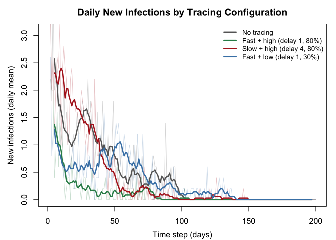
Without intervention the epidemic infects 66.8% of the population. Isolation alone brings that to 59.1%, a modest change for a program that diagnoses 50% of symptomatic cases, because most transmission has already happened by the time a case is diagnosed. Adding tracing with fast, high-coverage reach brings the attack rate to 41.7%; the slow program at the same coverage reaches 43.3% and the fast program at low coverage 50.5%. The intervals and ranges say how much of those differences the ten simulations can resolve, and the averted-infections table below puts an interval on each difference directly.
Where transmission comes from
The transmission record is the check that the natural history does what the parameter table claims, and it shows what each intervention leaves untouched.
source_tbl <- t(sapply(res, function(r) {
  c(round(100 * as.numeric(r$stage_share)),
    round(100 * r$restricted_share),
    round(r$r_seed, 2), round(r$gen_time, 1))
}))
colnames(source_tbl) <- c("Presymptomatic (%)", "Symptomatic (%)",
                          "Asymptomatic (%)", "Under isolation or quarantine (%)",
                          "Secondary infections per seed", "Generation time (days)")
knitr::kable(source_tbl,
caption = "Share of all transmissions by the infector's substage and by whether the infector was isolated or either partner quarantined; mean secondary infections generated by each seed; and mean generation time (days from the infector's infection to the infectee's), pooled over simulations")| Presymptomatic (%) | Symptomatic (%) | Asymptomatic (%) | Under isolation or quarantine (%) | Secondary infections per seed | Generation time (days) | |
|---|---|---|---|---|---|---|
| none | 40 | 42 | 18 | 0 | 1.69 | 8.4 |
| iso | 43 | 37 | 21 | 3 | 1.59 | 8.3 |
| fast_high | 43 | 37 | 21 | 12 | 1.69 | 8.5 |
| slow_high | 44 | 37 | 20 | 10 | 1.63 | 8.3 |
| fast_low | 43 | 37 | 20 | 7 | 1.46 | 8.5 |
In the no-intervention scenario 40% of transmissions come from presymptomatic infectors and 18% from asymptomatic ones, so symptom-based isolation can act on at most the remaining 42%, and only on the diagnosed half of those. Among transmissions from infections that go on to develop symptoms, 49% occur before onset, a little above the 45% that the stage durations and multipliers imply for an infector whose partners all remain susceptible, because partners infected during the presymptomatic stage are no longer at risk during the symptomatic one. The seeds generate 1.69 secondary infections each in a fully susceptible population. The mean generation time is 8.4 days, longer than the 5 to 6.5 days estimated for the wild-type virus. Geometric stage durations have long right tails, and within a geometric stage a transmission is as likely late as early, so a model with geometric stages cannot match the incubation period, the presymptomatic share, and the generation time all at once; this one sacrifices the last, and its epidemic is correspondingly slower than a real one with the same reproduction number. Under isolation the presymptomatic share rises, because isolation removes symptomatic transmission and nothing else. Under tracing a growing share of the remaining transmissions happens across edges where someone was isolated or quarantined: the leakage of imperfect restriction.
Infections averted and what they cost
Each tracing scenario is compared with isolation only, the program it adds to, on per-simulation infection counts, with a 95% Monte Carlo interval from the between-simulation variance of the two arms. The cost side is read from the same simulations: contacts found per index, the share of those found through partnerships that had already ended (the part of the program that the cumulative edgelist alone makes possible), the number of people quarantined, quarantine person-days per infection averted, and the peak share of the population in quarantine.
trace_scn <- c("fast_high", "slow_high", "fast_low")
averted <- lapply(trace_scn, function(s) mc_diff(res$iso$cum_inf, res[[s]]$cum_inf))
names(averted) <- trace_scn
speed_diff <- mc_diff(res$slow_high$cum_inf, res$fast_high$cum_inf)
coverage_diff <- mc_diff(res$fast_low$cum_inf, res$fast_high$cum_inf)

int_tbl <- data.frame(
  Scenario = labels[trace_scn],
  `Infections averted` = sapply(averted, fmt_ci, digits = 0),
  `Percent of isolation-only infections` = sapply(trace_scn, function(s)
    round(100 * averted[[s]]["est"] / mean(res$iso$cum_inf), 1)),
  `Contacts per index` = sapply(trace_scn, function(s)
    round(sum(res[[s]]$part) / sum(res[[s]]$index), 1)),
  `Ended partnerships (%)` = sapply(trace_scn, function(s)
    round(100 * sum(res[[s]]$part_ended) / sum(res[[s]]$part))),
  `Quarantine episodes` = sapply(trace_scn, function(s) round(mean(res[[s]]$quar_start))),
  `Quarantine days per infection averted` = sapply(trace_scn, function(s)
    round(mean(res[[s]]$quar_days) / averted[[s]]["est"])),
  `Peak share of population in quarantine (%)` = sapply(trace_scn, function(s)
    round(max(res[[s]]$quar_pct), 1)),
  check.names = FALSE, row.names = NULL
)
knitr::kable(int_tbl,
caption = "Infections averted relative to isolation only (mean and 95% Monte Carlo interval), the contacts found per traced index and the share found through ended partnerships, quarantine episodes started per simulation, quarantine person-days per infection averted, and the peak share of the population in quarantine")| Scenario | Infections averted | Percent of isolation-only infections | Contacts per index | Ended partnerships (%) | Quarantine episodes | Quarantine days per infection averted | Peak share of population in quarantine (%) |
|---|---|---|---|---|---|---|---|
| Tracing: fast (1 d), 80% reached | 870 (775, 965) | 29.4 | 9.8 | 51 | 5330 | 63 | 9.2 |
| Tracing: slow (4 d), 80% reached | 790 (696, 884) | 26.7 | 9.7 | 69 | 5307 | 70 | 11.7 |
| Tracing: fast (1 d), 30% reached | 433 (337, 529) | 14.6 | 9.6 | 50 | 2468 | 57 | 4.9 |
par(mfrow = c(1, 2), mar = c(8, 4.5, 3, 1), mgp = c(3, 0.8, 0))
short <- c(fast_high = "Fast, 80%", slow_high = "Slow, 80%", fast_low = "Fast, 30%")
av_est <- sapply(averted, function(v) 100 * v["est"] / N)
av_lo <- sapply(averted, function(v) 100 * v["lo"] / N)
av_hi <- sapply(averted, function(v) 100 * v["hi"] / N)
bp <- barplot(av_est, names.arg = short[trace_scn], col = cols[trace_scn], las = 2,
              ylab = "Infections averted per 100 population",
              main = "Averted vs Isolation Only",
              ylim = c(min(0, av_lo, av_est, na.rm = TRUE),
                       max(0, av_est, av_hi, na.rm = TRUE) * 1.2))
if (!all(is.na(av_lo))) arrows(bp, av_lo, bp, av_hi, angle = 90, code = 3, length = 0.04)
text(bp, pmax(av_hi, av_est, na.rm = TRUE) + max(c(av_est, av_hi), na.rm = TRUE) * 0.05,
     sprintf("%.1f", av_est), cex = 0.85, font = 2)
qd <- sapply(trace_scn, function(s) mean(res[[s]]$quar_days) / averted[[s]]["est"])
bp2 <- barplot(qd, names.arg = short[trace_scn], col = cols[trace_scn], las = 2,
               ylab = "Quarantine person-days per infection averted",
               main = "Cost of Averting One Infection",
               ylim = c(min(0, qd), max(0, qd) * 1.2))
text(bp2, qd + max(qd) * 0.05, sprintf("%.0f", qd), cex = 0.85, font = 2)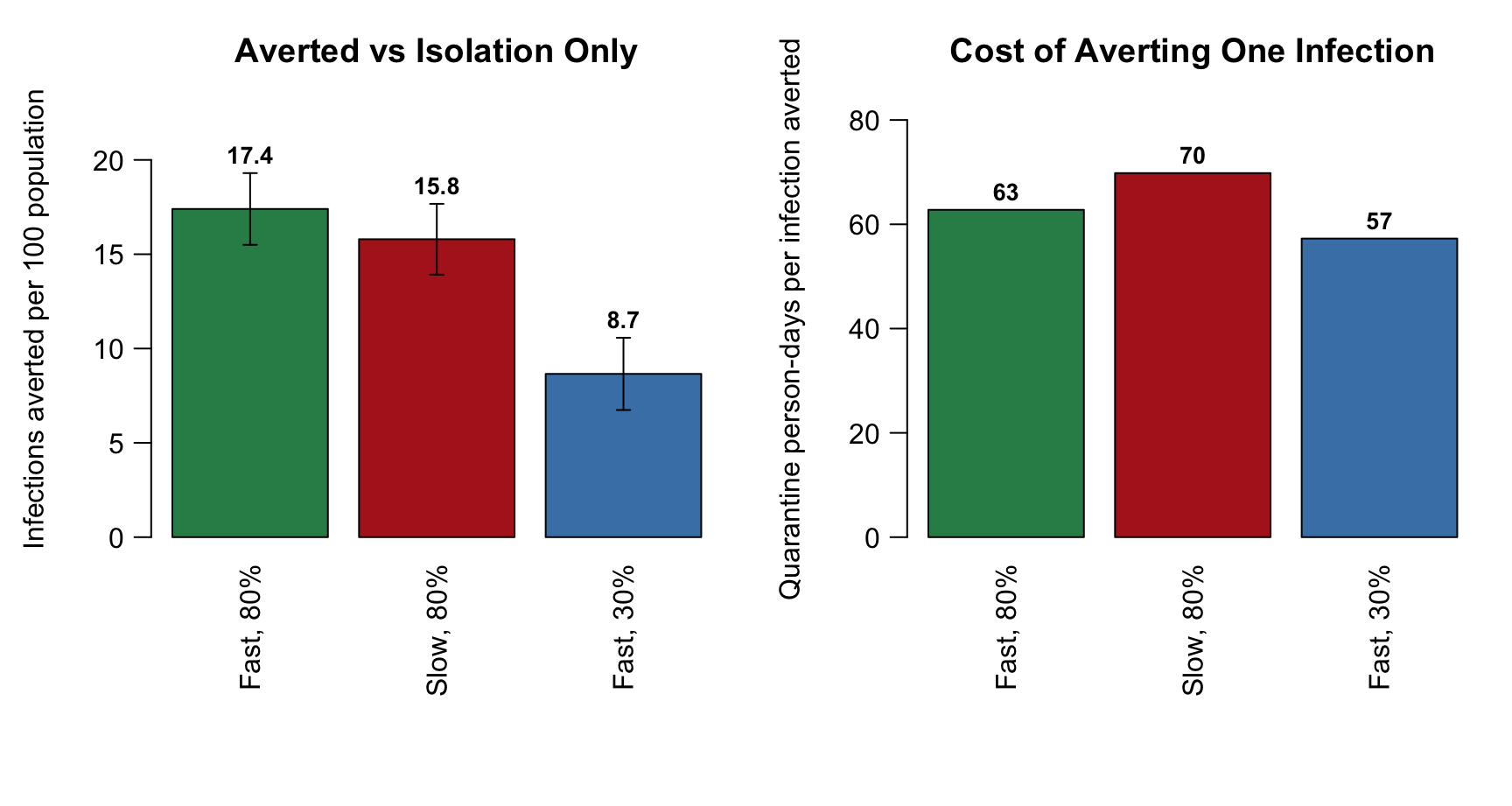
Coverage is the larger lever. Cutting reach from 80% to 30% at the same speed gives up 50% of the infections averted, a difference of 437 (348, 527) infections between the two fast arms. Slowing the trace from 1 to 4 days at 80% reach changes the final size by 80 (-7, 168) infections, 18% of the coverage contrast and at the limit of what ten simulations resolve, and the two high-coverage arms start about the same number of quarantine episodes (5307 against 5330 per simulation). The low-coverage program averts 50% of what the fast, high-coverage program averts, from 46% as many quarantine episodes. The delay matters more for the shape of the epidemic than for its size: daily incidence under the fast program peaks at 17 new infections, against 23 under the slow one (7-day average of the mean across simulations). It also changes which contacts the program finds, and the next section shows that directly.
The weak effect of the tracing delay on the final size differs from the branching-process results, where a delay of a few days is decisive (Kretzschmar et al. 2020), and the difference is instructive rather than a contradiction. Those models count only the transmissions prevented from the index’s infected contacts, for which every day of delay matters because the contacts are progressing through their latent period. In this population model most reached contacts are susceptible, and quarantining them protects them from everyone else for ten days regardless of how promptly they were reached. At the incidence in these simulations, 9.2% of the population is in quarantine at the peak of the fast, high-coverage program, and that population-level distancing, not the timing of individual quarantines, is where most of the effect comes from. The per-index mechanism is still there: it is what separates the fast and slow programs in the latent-contact yield below, and it would dominate at lower incidence, where few people are quarantined at once. The Kucharski et al. 2020 and Firth et al. results, which report tens of contacts quarantined per case and large shares of a population in quarantine, are the same effect seen from the burden side.
What a tracer finds
The state a reached contact was in when reached is the yield of the program. Only latent and infectious contacts can have their onward transmission reduced; susceptible contacts are protected while quarantined, and recovered contacts are quarantined for nothing. Partners who had themselves already been diagnosed are excluded before reach, here and in the contacts-per-index column above, so the recovered share is that of never-diagnosed contacts.
yield <- sapply(trace_scn, function(s) {
  m <- colSums(res[[s]]$reach_state)
  100 * m / sum(m)
})
yield_tbl <- data.frame(
  Scenario = labels[trace_scn],
  `Contacts reached` = sapply(trace_scn, function(s) round(mean(res[[s]]$reach))),
  `Susceptible (%)` = round(yield["s", ], 1),
  `Latent (%)` = round(yield["e", ], 1),
  `Infectious (%)` = round(yield["i", ], 1),
  `Recovered (%)` = round(yield["r", ], 1),
  check.names = FALSE, row.names = NULL
)
knitr::kable(yield_tbl,
caption = "Contacts reached per simulation and their disease state on the day they were reached, percent of all reached contacts, pooled over simulations")| Scenario | Contacts reached | Susceptible (%) | Latent (%) | Infectious (%) | Recovered (%) |
|---|---|---|---|---|---|
| Tracing: fast (1 d), 80% reached | 5752 | 71.5 | 2.9 | 7.5 | 18.1 |
| Tracing: slow (4 d), 80% reached | 5833 | 69.6 | 1.8 | 7.0 | 21.6 |
| Tracing: fast (1 d), 30% reached | 2577 | 66.3 | 3.5 | 8.9 | 21.3 |
par(mfrow = c(1, 1), mar = c(4, 4.5, 3, 1), mgp = c(2.6, 0.8, 0))
ycols <- c(s = "#3498db", e = "#8e44ad", i = "#e74c3c", r = "#27ae60")
bp3 <- barplot(yield, names.arg = short[trace_scn], col = ycols, las = 1,
               ylab = "Percent of reached contacts", ylim = c(0, 118),
               main = "State of Contacts When Reached")
legend("top", horiz = TRUE, bty = "n", fill = ycols, cex = 0.85,
       legend = c("Susceptible", "Latent", "Infectious", "Recovered"))
text(bp3, 100 - yield["s", ] / 2, sprintf("%.0f%%", yield["s", ]), col = "white")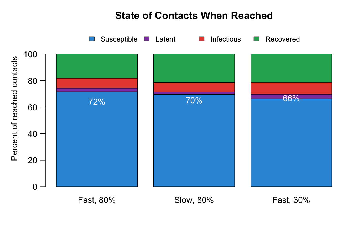
About 10% of the contacts the fast program reaches carry an active infection, latent or infectious, on the day they are reached, and about 18% have already recovered. The active-infection share is a point prevalence rather than a secondary attack rate, but it sits where program data put the yield of tracing: a 6% secondary attack rate among app-notified contacts (Wymant et al. 2021) and 19% test positivity among traced household contacts (Kerr et al. 2021). The slow program’s yield is the timing mechanism made visible: it reaches 1.8% latent contacts against the fast program’s 2.9%, the contacts for whom quarantine prevents the most transmission, and more already-recovered contacts (22% against 18%), for whom it prevents none. Three extra days of delay convert latent contacts into recovered ones.
Burden over time
par(mfrow = c(1, 1), mar = c(4, 4.2, 2.5, 1), mgp = c(2.4, 0.8, 0))
restricted <- lapply(sims, function(sim) {
  df <- as.data.frame(sim)
  100 * tapply(df$iso.num + df$quar.num, df$time, mean) / N
})
plot(NA, xlim = c(1, nsteps), ylim = c(0, max(sapply(restricted, max, na.rm = TRUE)) * 1.1),
     xlab = "Day", ylab = "Percent of population isolated or quarantined",
     main = "Population Under Movement Restriction")
for (s in names(sims)) {
  lines(as.numeric(names(restricted[[s]])), restricted[[s]], lwd = 2, col = cols[s])
}
legend("topright", legend = labels, col = cols, lwd = 2, bty = "n", cex = 0.75)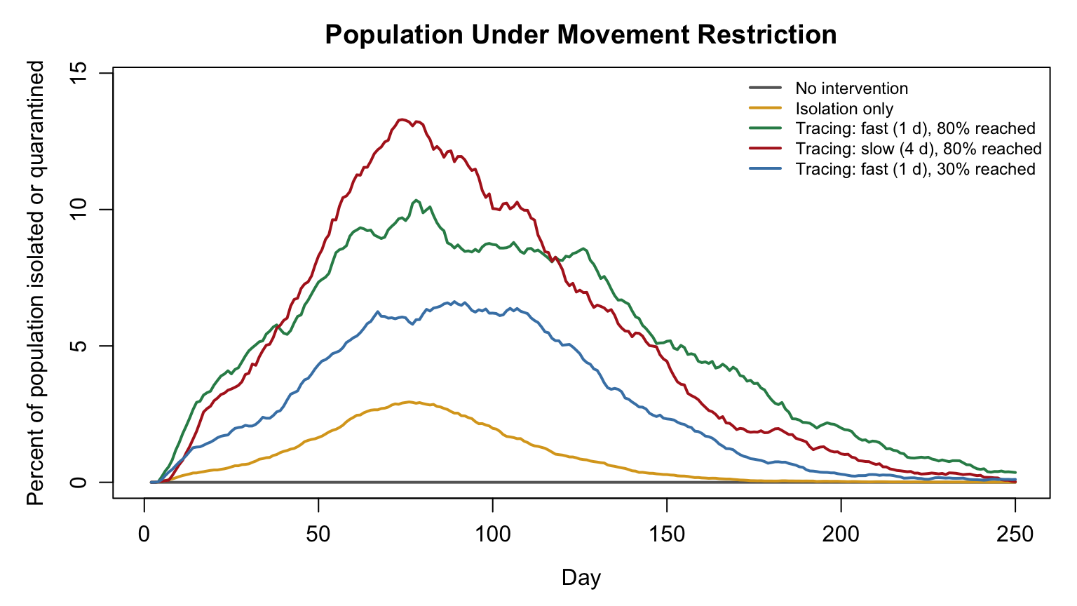
The curve is the program’s footprint. It scales with incidence times contacts per index times quarantine length, which is why a tracing program’s burden peaks with the epidemic it is trying to suppress and why programs without a capacity limit, like this one, are optimistic about what could be delivered at the peak. The area under the tracing curves, divided by the infections each averted, is the person-days column of the averted table.
Between-simulation variability
cv_tbl <- t(sapply(res, function(r) {
  c(`Mean attack rate (%)` = round(mean(r$attack), 1),
    CV = round(sd(r$attack) / mean(r$attack), 2))
}))
knitr::kable(cv_tbl, caption = "Coefficient of variation of the attack rate across simulations, by scenario")| Mean attack rate (%) | CV | |
|---|---|---|
| none | 66.8 | 0.02 |
| iso | 59.1 | 0.04 |
| fast_high | 41.7 | 0.05 |
| slow_high | 43.3 | 0.05 |
| fast_low | 50.5 | 0.04 |
The no-intervention and isolation-only epidemics are large and their final sizes vary little between simulations. The tracing scenarios are closer to the epidemic threshold, where final sizes vary more relative to their mean, which is the honest state of any comparison between interventions that hold an epidemic near criticality. With ten simulations the intervals separate the coverage contrast cleanly and leave the speed contrast at the limit of resolution; more simulations narrow them in proportion to the square root of their number, and the run time scales linearly.
Next Steps
- Test the reached contacts. Add a parameter
test.contactsand, in step 5 oftrace, diagnose reached contacts who are latent or infectious with a test sensitivity, settingdx.timeandiso.untilfor the positives. They then become indices for the next generation of tracing, and asymptomatic infections become findable. The yield table shows how many the test would find. - A capacity limit. Cap the number of indices traced per day (for example a fixed share of the population) and drop or queue the rest. This is the constraint that broke programs in 2020, and it turns the burden curve into a design input.
- Testing delay against tracing delay. Vary
dx.delaybetween 1 and 6 days alongsidetrace.delay. In the branching-process literature the testing delay is the binding constraint; this model can say how that plays out at the population level, where the quarantine of susceptible contacts does not depend on either delay. - A lower-incidence regime. Reduce
inf.probor the seed count so that few people are in quarantine at once, and compare the speed and coverage effects with those here. The per-index mechanism should become visible in the final sizes as the population-level effect shrinks. - Households. Add a household clique layer (see RSV) so that household contacts, which are the most likely to be infected and the easiest to reach, can be traced with certainty and community contacts with the reach probability.
get_partners()takes anetworksargument for layer-specific lookups. - Backward tracing. The elicitation window here runs forward from 2 days before onset. Extending it back through the index’s incubation period looks for the index’s own infector, whose other contacts are the highest-yield targets when transmission is overdispersed (Bradshaw et al. 2021; Kojaku et al. 2021). On this network with a Poisson degree distribution the gain would be small; add degree heterogeneity to the formation model and it grows.
- Adherence as a draw rather than a multiplier. Replace
quar.multwith a per-contact Bernoulli adherence draw, so that some contacts quarantine fully and others not at all, and compare with the mean-multiplier version here. Surveyed adherence in 2020 was far below the 70% assumed (Smith et al. 2021; Davis et al. 2021).
References
Contact tracing models:
- Fraser C, Riley S, Anderson RM, Ferguson NM. (2004). Factors that make an infectious disease outbreak controllable. Proc Natl Acad Sci U S A 101(16):6146-6151. https://doi.org/10.1073/pnas.0307506101
- Eames KTD, Keeling MJ. (2003). Contact tracing and disease control. Proc R Soc Lond B 270(1533):2565-2571. https://doi.org/10.1098/rspb.2003.2554
- House T, Keeling MJ. (2010). The impact of contact tracing in clustered populations. PLoS Comput Biol 6(3):e1000721. https://doi.org/10.1371/journal.pcbi.1000721
- Hellewell J, Abbott S, Gimma A, et al. (2020). Feasibility of controlling COVID-19 outbreaks by isolation of cases and contacts. Lancet Glob Health 8(4):e488-e496. https://doi.org/10.1016/S2214-109X(20)30074-7
- Kretzschmar ME, Rozhnova G, Bootsma MCJ, van Boven M, van de Wijgert JHHM, Bonten MJM. (2020). Impact of delays on effectiveness of contact tracing strategies for COVID-19: a modelling study. Lancet Public Health 5(8):e452-e459. https://doi.org/10.1016/S2468-2667(20)30157-2
- Kucharski AJ, Klepac P, Conlan AJK, et al. (2020). Effectiveness of isolation, testing, contact tracing, and physical distancing on reducing transmission of SARS-CoV-2 in different settings: a mathematical modelling study. Lancet Infect Dis 20(10):1151-1160. https://doi.org/10.1016/S1473-3099(20)30457-6
- Firth JA, Hellewell J, Klepac P, Kissler S, CMMID COVID-19 Working Group, Kucharski AJ, Spurgin LG. (2020). Using a real-world network to model localized COVID-19 control strategies. Nat Med 26(10):1616-1622. https://doi.org/10.1038/s41591-020-1036-8
- Kerr CC, Mistry D, Stuart RM, et al. (2021). Controlling COVID-19 via test-trace-quarantine. Nat Commun 12(1):2993. https://doi.org/10.1038/s41467-021-23276-9
- Bradshaw WJ, Alley EC, Huggins JH, Lloyd AL, Esvelt KM. (2021). Bidirectional contact tracing could dramatically improve COVID-19 control. Nat Commun 12(1):232. https://doi.org/10.1038/s41467-020-20325-7
- Kojaku S, Hébert-Dufresne L, Mones E, Lehmann S, Ahn YY. (2021). The effectiveness of backward contact tracing in networks. Nat Phys 17(6):652-658. https://doi.org/10.1038/s41567-021-01187-2
- Davis EL, Lucas TCD, Borlase A, et al. (2021). Contact tracing is an imperfect tool for controlling COVID-19 transmission and relies on population adherence. Nat Commun 12(1):5412. https://doi.org/10.1038/s41467-021-25531-5
- Quilty BJ, Clifford S, Hellewell J, et al. (2021). Quarantine and testing strategies in contact tracing for SARS-CoV-2: a modelling study. Lancet Public Health 6(3):e175-e183. https://doi.org/10.1016/S2468-2667(20)30308-X
- Müller J, Kretzschmar M. (2021). Contact tracing: old models and new challenges. Infect Dis Model 6:222-231. https://doi.org/10.1016/j.idm.2020.12.005
Natural history:
- Lauer SA, Grantz KH, Bi Q, et al. (2020). The incubation period of coronavirus disease 2019 (COVID-19) from publicly reported confirmed cases: estimation and application. Ann Intern Med 172(9):577-582. https://doi.org/10.7326/M20-0504
- McAloon C, Collins Á, Hunt K, et al. (2020). Incubation period of COVID-19: a rapid systematic review and meta-analysis of observational research. BMJ Open 10(8):e039652. https://doi.org/10.1136/bmjopen-2020-039652
- He X, Lau EHY, Wu P, et al. (2020). Temporal dynamics in viral shedding and transmissibility of COVID-19. Nat Med 26(5):672-675. https://doi.org/10.1038/s41591-020-0869-5. Author correction: Nat Med 26(9):1491-1493. https://doi.org/10.1038/s41591-020-1016-z
- Ferretti L, Wymant C, Kendall M, et al. (2020). Quantifying SARS-CoV-2 transmission suggests epidemic control with digital contact tracing. Science 368(6491):eabb6936. https://doi.org/10.1126/science.abb6936
- van Kampen JJA, van de Vijver DAMC, Fraaij PLA, et al. (2021). Duration and key determinants of infectious virus shedding in hospitalized patients with coronavirus disease-2019 (COVID-19). Nat Commun 12(1):267. https://doi.org/10.1038/s41467-020-20568-4
- Cevik M, Tate M, Lloyd O, Maraolo AE, Schafers J, Ho A. (2021). SARS-CoV-2, SARS-CoV, and MERS-CoV viral load dynamics, duration of viral shedding, and infectiousness: a systematic review and meta-analysis. Lancet Microbe 2(1):e13-e22. https://doi.org/10.1016/S2666-5247(20)30172-5
- Buitrago-Garcia D, Ipekci AM, Heron L, et al. (2022). Occurrence and transmission potential of asymptomatic and presymptomatic SARS-CoV-2 infections: update of a living systematic review and meta-analysis. PLoS Med 19(5):e1003987. https://doi.org/10.1371/journal.pmed.1003987
- Sah P, Fitzpatrick MC, Zimmer CF, et al. (2021). Asymptomatic SARS-CoV-2 infection: a systematic review and meta-analysis. Proc Natl Acad Sci U S A 118(34):e2109229118. https://doi.org/10.1073/pnas.2109229118
- Sayampanathan AA, Heng CS, Pin PH, Pang J, Leong TY, Lee VJ. (2021). Infectivity of asymptomatic versus symptomatic COVID-19. Lancet 397(10269):93-94. https://doi.org/10.1016/S0140-6736(20)32651-9
- Billah MA, Miah MM, Khan MN. (2020). Reproductive number of coronavirus: a systematic review and meta-analysis based on global level evidence. PLoS One 15(11):e0242128. https://doi.org/10.1371/journal.pone.0242128
Program performance and guidance:
- Lash RR, Moonan PK, Byers BL, et al. (2021). COVID-19 case investigation and contact tracing in the US, 2020. JAMA Netw Open 4(6):e2115850. https://doi.org/10.1001/jamanetworkopen.2021.15850
- Smith LE, Potts HWW, Amlôt R, Fear NT, Michie S, Rubin GJ. (2021). Adherence to the test, trace, and isolate system in the UK: results from 37 nationally representative surveys. BMJ 372:n608. https://doi.org/10.1136/bmj.n608
- Wymant C, Ferretti L, Tsallis D, et al. (2021). The epidemiological impact of the NHS COVID-19 app. Nature 594(7863):408-412. https://doi.org/10.1038/s41586-021-03606-z
- CDC. Contact tracing for COVID-19: appendix and glossary of key terms (archived). https://archive.cdc.gov/www_cdc_gov/coronavirus/2019-ncov/php/contact-tracing/contact-tracing-plan/appendix.html
- CDC. (December 2, 2020). Options to reduce quarantine for contacts of persons with SARS-CoV-2 infection using symptom monitoring and diagnostic testing. https://www.ncbi.nlm.nih.gov/books/NBK570434/
The network, transmission probability, ascertainment, delays, and restriction multipliers are illustrative choices, selected to place the model in the regime where contact tracing is used and to reproduce the qualitative natural history of the wild-type virus. They are not calibrated to any outbreak.