flowchart LR
    S["<b>S</b><br/>Susceptible"] -->|"infection<br/>(si.flow)"| I
    I["<b>I</b><br/>Infectious"] -->|"recovery<br/>(ir.flow)"| R["<b>R</b><br/>Recovered"]
    S -->|"vaccination<br/>(sv.flow, schedule-gated)"| V["<b>V</b><br/>Vaccine-Immune"]
    R -.->|"waning<br/>(rs.flow, optional)"| S
    V -.->|"waning<br/>(vs.flow, optional)"| S

    style S fill:#3498db,color:#fff
    style I fill:#e74c3c,color:#fff
    style R fill:#27ae60,color:#fff
    style V fill:#8e44ad,color:#fff
SIR with Time-Varying (Phased) Vaccination
SIR
SIRS
vaccination
intervention timing
reactive
intermediate
Phased and reactive vaccination on an SIR network model, with a bonus endemic-SIRS scenario where the reactive program produces sustained on/off cycling.
Overview
Every other intervention example in the Gallery applies its intervention from the start of the simulation and never stops. Real public health interventions almost never look like that. Campaigns begin on specific dates, policies are enacted and later relaxed, and reactive programs activate only when disease activity crosses a threshold. This example demonstrates how to implement time-varying interventions in EpiModel: interventions whose activity flips on or off based on the current timestep, on a more complex schedule of windows, or on the current state of the epidemic itself.
The disease model is a standard SIR on a 500-node contact network. A custom vaccinate module reads an activation schedule from the parameter set and applies vaccination only when the schedule says it is active. The same module supports two scheduling styles with no code changes: windowed schedules (one or more time intervals during which vaccination is active) and reactive schedules (activation triggered by prevalence crossing thresholds, with hysteresis to prevent rapid on/off flapping).
Five closed-SIR scenarios share identical disease parameters and the same per-timestep vaccination rate; they differ only in their activation schedule. Two further scenarios switch on slow waning of natural and vaccine immunity, converting the model to an endemic SIRS setting where the reactive program demonstrates sustained on/off cycling across a long horizon. That endemic comparison is the most striking phenomenon in this example: the same control logic that produces a one-shot mop-up on a closed SIR turns into a closed-loop adaptive intervention when the disease is genuinely endemic.
TipDownload standalone scripts
- model.R — Main simulation script
- module-fx.R — Custom module functions
Model Structure
| Compartment | Label | Description |
|---|---|---|
| Susceptible | S | Not infected; at risk of exposure |
| Infectious | I | Infected and can transmit to contacts |
| Recovered | R | Recovered from infection; immune (permanent if rs.rate = 0) |
| Vaccine-immune | V | Vaccinated and protected (permanent if vax.wane = 0) |
The vaccination flow is the only one whose rate varies with at — everything else behaves like a standard SIR (or SIRS, when waning is enabled). Solid arrows are the closed-SIR flows; dashed arrows are the optional waning paths that switch the model into the endemic regime.
The Time-Varying Intervention Pattern
The pedagogical core of this example is a small, reusable code pattern. Each timestep the module asks a single question: is the intervention active right now? The answer flips a binary vax.active flag, and the vaccination probability is multiplied by that flag.
# Windowed schedule: active if `at` lies inside any (start, end) window
vax.active <- any(at >= vax.starts & at <= vax.ends)

# Reactive schedule: hysteresis-based activation on current prevalence
if (prev.active == 1) {
  vax.active <- current.prev > vax.prev.off
} else {
  vax.active <- current.prev > vax.prev.on
}
The same pattern generalizes to any time-varying or state-dependent intervention: a time-limited treatment program, capacity-constrained testing, seasonal control measures, or an isolation policy triggered when ICU occupancy rises. The disease model never has to know about the schedule; it lives entirely inside the intervention module.
Setup
suppressMessages(library(EpiModel))

nsims <- 5
ncores <- 5
nsteps <- 400
nsteps_endemic <- 1000
Custom Modules
Infection Module
Standard S to I transmission along discordant edges, plus an optional exog.inf.prob parameter that adds an external (exogenous) force of infection. At each timestep every active susceptible has probability exog.inf.prob of being infected by a source outside the modeled network: spillover from an unmodeled reservoir, environmental exposure, or contacts with individuals not represented in the simulated network. This is distinct from importation, which describes already-infected individuals arriving in the population and is properly modeled as an arrivals process in a vital-dynamics module. Here the population is closed and existing susceptibles transition to infectious at a constant background hazard, independent of in-population prevalence. Vaccine-immune individuals (status == "v") are excluded automatically because discord_edgelist() only pairs "s" with "i".
infect <- function(dat, at) {

  active <- get_attr(dat, "active")
  status <- get_attr(dat, "status")
  infTime <- get_attr(dat, "infTime")

  inf.prob <- get_param(dat, "inf.prob")
  act.rate <- get_param(dat, "act.rate")
  exog.inf.prob <- get_param(dat, "exog.inf.prob")

  idsInf <- which(active == 1 & status == "i")
  nActive <- sum(active == 1)
  nElig <- length(idsInf)
  nInf <- 0
  nExog <- 0

  ## Endogenous network transmission ##
  if (nElig > 0 && nElig < nActive) {
1    del <- discord_edgelist(dat, at)
    if (!is.null(del) && nrow(del) > 0) {
      del$transProb <- inf.prob
      del$actRate <- act.rate
      del$finalProb <- 1 - (1 - del$transProb)^del$actRate
      transmit <- rbinom(nrow(del), 1, del$finalProb)
      del <- del[which(transmit == 1), ]
      idsNewInf <- unique(del$sus)
      nInf <- length(idsNewInf)
      if (nInf > 0) {
        status[idsNewInf] <- "i"
        infTime[idsNewInf] <- at
      }
    }
  }

  ## Exogenous force of infection ##
2  if (exog.inf.prob > 0) {
    idsSus <- which(active == 1 & status == "s")
    if (length(idsSus) > 0) {
      vecExog <- which(rbinom(length(idsSus), 1, exog.inf.prob) == 1)
      nExog <- length(vecExog)
      if (nExog > 0) {
        idsExog <- idsSus[vecExog]
        status[idsExog] <- "i"
        infTime[idsExog] <- at
      }
    }
  }

  if (nInf + nExog > 0) {
    dat <- set_attr(dat, "status", status)
    dat <- set_attr(dat, "infTime", infTime)
  }

  dat <- set_epi(dat, "si.flow", at, nInf)
  dat <- set_epi(dat, "exog.flow", at, nExog)
  return(dat)
}- 1
-
discord_edgelist()only considers nodes with status"s"or"i". Vaccine-immune individuals ("v") and recovered individuals ("r") never appear and are therefore protected without any explicit exclusion logic. - 2
-
The exogenous force of infection adds a constant per-step Bernoulli hazard to every susceptible (e.g. spillover from an unmodeled reservoir, environmental exposure, off-network contacts). Setting
exog.inf.prob = 0gives a purely network-driven model. This is not importation, which would describe already-infected individuals arriving in the population and is properly handled by an arrivals module.
Recovery Module
Two flows: I to R at rec.rate, plus an optional R to S waning of natural immunity at rs.rate. When rs.rate = 0 this is standard SIR; when rs.rate > 0 it becomes SIRS.
recov <- function(dat, at) {

  active <- get_attr(dat, "active")
  status <- get_attr(dat, "status")
  rec.rate <- get_param(dat, "rec.rate")
  rs.rate <- get_param(dat, "rs.rate")

  ## I -> R ##
  nRec <- 0
  idsElig <- which(active == 1 & status == "i")
  if (length(idsElig) > 0) {
    vec <- which(rbinom(length(idsElig), 1, rec.rate) == 1)
    if (length(vec) > 0) {
      idsRec <- idsElig[vec]
      nRec <- length(idsRec)
      status[idsRec] <- "r"
    }
  }

  ## R -> S waning (optional, SIRS) ##
  nWane <- 0
1  if (rs.rate > 0) {
    idsEligWane <- which(active == 1 & status == "r")
    if (length(idsEligWane) > 0) {
      vecWane <- which(rbinom(length(idsEligWane), 1, rs.rate) == 1)
      if (length(vecWane) > 0) {
        idsWane <- idsEligWane[vecWane]
        nWane <- length(idsWane)
        status[idsWane] <- "s"
      }
    }
  }

  dat <- set_attr(dat, "status", status)
  dat <- set_epi(dat, "ir.flow", at, nRec)
  dat <- set_epi(dat, "rs.flow", at, nWane)
  dat <- set_epi(dat, "r.num", at, sum(active == 1 & status == "r"))
  return(dat)
}- 1
-
The
rs.rate > 0switch is what converts SIR to SIRS. It’s the single mechanism that lets the disease persist endemically and gives the reactive program something to keep responding to over a long horizon.
Vaccination Module
The schedule-driven module. The first block applies optional vaccine waning (V to S). The second decides whether the program is active at this timestep. The third is a standard all-or-nothing vaccination process, gated by the active flag.
vaccinate <- function(dat, at) {

  active <- get_attr(dat, "active")
  status <- get_attr(dat, "status")
  vax.attempted <- get_attr(dat, "vax.attempted",
                            override.null.error = TRUE)

  vax.rate <- get_param(dat, "vax.rate")
  vax.efficacy <- get_param(dat, "vax.efficacy")
  vax.wane <- get_param(dat, "vax.wane")
  vax.starts <- get_param(dat, "vax.starts")
  vax.ends <- get_param(dat, "vax.ends")
  vax.prev.on <- get_param(dat, "vax.prev.on")
  vax.prev.off <- get_param(dat, "vax.prev.off")

1  if (is.null(vax.attempted)) {
    vax.attempted <- rep(0, length(active))
    dat <- set_attr(dat, "vax.attempted", vax.attempted)
  }

  ## V -> S waning (optional) ##
  # Runs before the activity check so newly waned individuals are eligible
  # for re-vaccination in this same timestep if the program is active.
  nWane <- 0
  if (vax.wane > 0) {
    idsEligWane <- which(active == 1 & status == "v")
    if (length(idsEligWane) > 0) {
      vecWane <- which(rbinom(length(idsEligWane), 1, vax.wane) == 1)
      if (length(vecWane) > 0) {
        idsWane <- idsEligWane[vecWane]
        nWane <- length(idsWane)
        status[idsWane] <- "s"
2        vax.attempted[idsWane] <- 0
      }
    }
  }

  ## Activity check ##
3  if (vax.prev.on > 0) {
    nAct <- sum(active == 1)
    current.prev <- if (nAct > 0) {
      sum(active == 1 & status == "i") / nAct
    } else 0
    prev.active <- 0
    if (at > 2) {
      val <- get_epi(dat, "vax.active", at = at - 1,
                     override.null.error = TRUE)
      if (!is.null(val) && !is.na(val)) prev.active <- val
    }
    if (prev.active == 1) {
4      vax.active <- as.numeric(current.prev > vax.prev.off)
    } else {
      vax.active <- as.numeric(current.prev > vax.prev.on)
    }
  } else {
5    vax.active <- as.numeric(any(at >= vax.starts & at <= vax.ends))
  }

  ## Apply vaccination when active ##
  nVax <- 0
  nImmune <- 0
  if (vax.active == 1 && vax.rate > 0) {
    idsElig <- which(active == 1 & status == "s" & vax.attempted == 0)
    if (length(idsElig) > 0) {
      vecVax <- which(rbinom(length(idsElig), 1, vax.rate) == 1)
      if (length(vecVax) > 0) {
        idsVax <- idsElig[vecVax]
        nVax <- length(idsVax)
        vax.attempted[idsVax] <- 1
6        vecImmune <- which(rbinom(nVax, 1, vax.efficacy) == 1)
        idsImmune <- idsVax[vecImmune]
        nImmune <- length(idsImmune)
        if (nImmune > 0) status[idsImmune] <- "v"
      }
    }
  }

  dat <- set_attr(dat, "status", status)
  dat <- set_attr(dat, "vax.attempted", vax.attempted)

  dat <- set_epi(dat, "vax.active", at, vax.active)
  dat <- set_epi(dat, "vax.flow", at, nVax)
  dat <- set_epi(dat, "sv.flow", at, nImmune)
  dat <- set_epi(dat, "vs.flow", at, nWane)
  dat <- set_epi(dat, "v.num", at, sum(active == 1 & status == "v"))
  return(dat)
}- 1
-
Lazy initialization of the per-node
vax.attemptedflag on the module’s first call. - 2
- When a vaccinated individual’s protection wanes, reset their attempted flag so they’re eligible to be re-vaccinated by future activations.
- 3
-
Reactive mode is selected by setting
vax.prev.on > 0. Otherwise the module falls back to the windowed schedule. - 4
- Hysteresis. If currently active, stay active until prevalence drops below the lower threshold. If currently inactive, stay inactive until prevalence rises above the upper threshold. This prevents rapid on/off toggling near a single threshold.
- 5
- Vectorized window check. Parallel vectors of starts and ends mean the same line handles a single campaign, a bounded short campaign, or arbitrarily many pulses.
- 6
-
All-or-nothing protection. Each vaccinated individual becomes immune with probability
vax.efficacy. Unprotected vaccinees stay susceptible but theirvax.attemptedflag is set so they won’t be re-vaccinated until their protection (if any) wanes.
Network Model
n <- 500
nw <- network_initialize(n)

formation <- ~edges
1target.stats <- c(round(1.5 * n / 2))

coef.diss <- dissolution_coefs(dissolution = ~offset(edges), duration = 60)
est <- netest(nw, formation, target.stats, coef.diss)- 1
- Mean degree = 1.5 (375 edges across 500 nodes). High enough that transmission isn’t bottlenecked by isolation, low enough that the dynamics remain clean. The intervention timing is the focus, not the network.
Network Diagnostics
dx <- netdx(est, nsims = nsims, ncores = ncores, nsteps = nsteps,
            nwstats.formula = ~edges + degree(0:3))
Network Diagnostics
-----------------------
- Simulating 5 networks
- Calculating formation statisticsprint(dx)EpiModel Network Diagnostics
=======================
Diagnostic Method: Dynamic
Simulations: 5
Time Steps per Sim: 400
Formation Diagnostics
-----------------------
Target Sim Mean Pct Diff Sim SE Z Score SD(Sim Means) SD(Statistic)
edges 375 374.030 -0.259 2.777 -0.349 6.842 16.326
degree0 NA 113.139 NA 1.857 NA 3.563 11.021
degree1 NA 164.802 NA 1.585 NA 2.886 12.055
degree2 NA 126.776 NA 1.042 NA 2.538 9.700
degree3 NA 62.927 NA 0.886 NA 3.159 8.399
Duration Diagnostics
-----------------------
Target Sim Mean Pct Diff Sim SE Z Score SD(Sim Means) SD(Statistic)
edges 60 59.618 -0.637 0.729 -0.524 1.601 3.438
Dissolution Diagnostics
-----------------------
Target Sim Mean Pct Diff Sim SE Z Score SD(Sim Means) SD(Statistic)
edges 0.017 0.017 -0.008 0 -0.009 0 0.007plot(dx)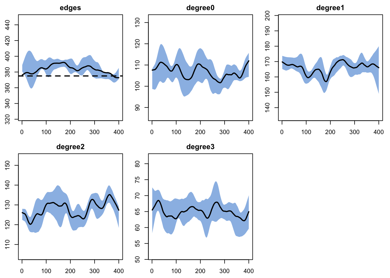
Epidemic Simulation
Control Settings
init <- init.net(i.num = 10)

control <- control.net(
  type = NULL,
  nsims = nsims,
  ncores = ncores,
  nsteps = nsteps,
  infection.FUN = infect,
  recovery.FUN = recov,
1  vaccinate.FUN = vaccinate,
  verbose = FALSE
)- 1
-
vaccinate.FUNis a custom module slot. Any name ending in.FUNcan be passed tocontrol.net()and EpiModel will splice it into the default module pipeline.
Base Parameters
All scenarios share the same disease parameters. The base parameter set holds defaults for every parameter the modules read; per-scenario overrides are applied via the scenarios API in the next section. vax.starts and vax.ends are length-2 vectors so the pulse scenario can express two activation windows via the _N vector-position suffix on the scenarios data frame.
- 1
-
rs.rate = 0keeps the model as standard SIR. Setting it positive switches on R-to-S waning (SIRS), which sustains an endemic equilibrium. - 2
-
vax.wane = 0keeps vaccine immunity permanent. Setting it positive lets vaccinated individuals return to the susceptible pool over time.
Closed-SIR Scenarios
Five scenarios share identical disease parameters and differ only in the activation schedule. The disease burns out as a single wave. Each scenario is one row in a flat data frame; the _1 and _2 columns encode positions of the length-2 vector parameters (an unused window position takes -1).
scenarios_sir.df <- data.frame(
  .scenario.id = c("none", "early", "late",  "pulse", "react"),
  .at          = 0,
  vax.rate     = c(0,      0.05,    0.05,    0.05,    0.05),
  vax.starts_1 = c(-1,     30,      100,     40,      -1),
  vax.starts_2 = c(-1,     -1,      -1,      120,     -1),
  vax.ends_1   = c(-1,     nsteps,  nsteps,  70,      -1),
  vax.ends_2   = c(-1,     -1,      -1,      150,     -1),
  vax.prev.on  = c(-1,     -1,      -1,      -1,      0.05),
  vax.prev.off = c(-1,     -1,      -1,      -1,      0.02)
)
scenarios_sir.list <- create_scenario_list(scenarios_sir.df)

sims <- list()
for (scn in scenarios_sir.list) {
  sims[[scn$id]] <- netsim(est, use_scenario(param_base, scn),
                           init, control)
}
Endemic SIRS Scenarios
Switching on rs.rate (natural immunity waning) and vax.wane (vaccine immunity waning) converts the model to a SIRS setting. The disease no longer burns out as a single wave; instead it settles into a sustained endemic equilibrium, and the reactive program acquires something to do over a long horizon.
control_endemic <- control.net(
  type = NULL,
  nsims = nsims,
  ncores = ncores,
  nsteps = nsteps_endemic,
  infection.FUN = infect,
  recovery.FUN = recov,
  vaccinate.FUN = vaccinate,
  verbose = FALSE
)

scenarios_endemic.df <- data.frame(
  .scenario.id = c("endemic_none", "endemic_react"),
  .at          = 0,
  vax.rate     = c(0,      0.07),
  rs.rate      = c(0.015,  0.015),
  vax.wane     = c(0.03,   0.03),
  vax.prev.on  = c(-1,     0.05),
  vax.prev.off = c(-1,     0.02)
)
scenarios_endemic.list <- create_scenario_list(scenarios_endemic.df)

sims_endemic <- list()
for (scn in scenarios_endemic.list) {
  sims_endemic[[scn$id]] <- netsim(est, use_scenario(param_base, scn),
                                   init, control_endemic)
}
sim_endemic_none <- sims_endemic[["endemic_none"]]
sim_endemic_react <- sims_endemic[["endemic_react"]]
Analysis
labels <- c(none = "No vaccination",
            early = "Early (start 30)",
            late = "Late (start 100)",
            pulse = "Pulses (40-70, 120-150)",
            react = "Reactive (>5% / <2%)")
cols <- c(none = "gray40", early = "seagreen", late = "firebrick",
          pulse = "#8e44ad", react = "steelblue")
sims <- lapply(sims, function(s) mutate_epi(s, prev = i.num / num))
Prevalence by Intervention Timing
Same disease, same per-step vaccination rate, different schedules. Early and Reactive both clip the epidemic peak; Late only mops up after the peak has passed; Pulses produce a knock-down/rebound shape as vaccination switches on and off.
par(mfrow = c(1, 1), mar = c(3, 3, 2, 1), mgp = c(2, 1, 0))
plot(sims$none, y = "prev",
     main = "Prevalence by Intervention Timing",
     ylab = "Prevalence (I / N)", xlab = "Time Step",
     mean.col = cols["none"], mean.lwd = 2, mean.smooth = TRUE,
     qnts = FALSE, legend = FALSE, ylim = ylim_epi(sims, "prev", qnts = FALSE))
for (k in c("early", "late", "pulse", "react")) {
  plot(sims[[k]], y = "prev",
       mean.col = cols[k], mean.lwd = 2, mean.smooth = TRUE,
       qnts = FALSE, legend = FALSE, add = TRUE)
}
legend("topright", legend = labels, col = cols, lwd = 2, bty = "n",
       cex = 0.8)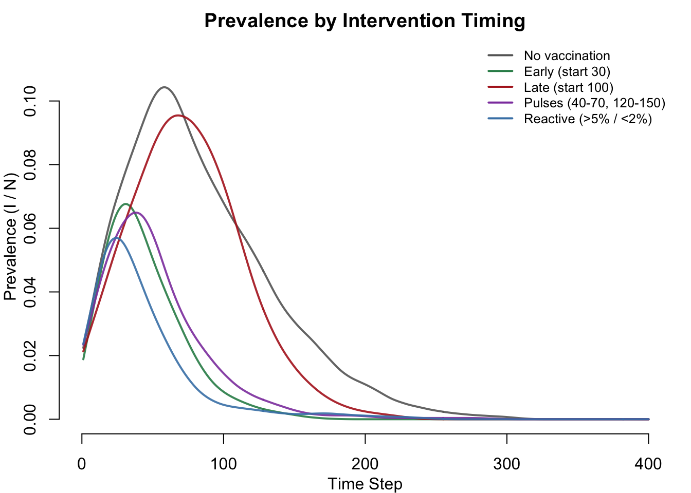
Disease Burden and Per-Dose Efficiency
The cumulative-burden bar chart shows the Early vs. Late contrast clearly. The per-dose efficiency plot tells a complementary story: the Reactive scenario uses far fewer doses to achieve a comparable reduction, and ends up with the highest infections averted per dose of any scenario.
cum_inf <- sapply(sims, function(s) {
  df <- as.data.frame(s)
  mean(tapply(df$si.flow, df$sim, sum, na.rm = TRUE))
})
total_vax <- sapply(sims, function(s) {
  df <- as.data.frame(s)
  mean(tapply(df$vax.flow, df$sim, sum, na.rm = TRUE))
})
averted <- cum_inf["none"] - cum_inf
avert_per_dose <- ifelse(total_vax > 0, averted / total_vax, NA)

par(mfrow = c(1, 2), mar = c(7, 4, 2, 1), mgp = c(2.5, 1, 0))
bp <- barplot(cum_inf, col = cols, las = 2,
              ylab = "Cumulative infections",
              main = "Disease Burden", names.arg = labels,
              cex.names = 0.8, ylim = c(0, max(cum_inf) * 1.15))
text(bp, cum_inf + max(cum_inf) * 0.03, round(cum_inf),
     cex = 0.8, font = 2)

apd_plot <- avert_per_dose
apd_plot[is.na(apd_plot)] <- 0
bp2 <- barplot(apd_plot, col = cols, las = 2,
               ylab = "Infections averted per dose",
               main = "Per-Dose Efficiency", names.arg = labels,
               cex.names = 0.8,
               ylim = c(0, max(apd_plot, na.rm = TRUE) * 1.15 + 0.01))
text(bp2, apd_plot + max(apd_plot, na.rm = TRUE) * 0.03,
     ifelse(is.na(avert_per_dose), "n/a", sprintf("%.2f", apd_plot)),
     cex = 0.8, font = 2)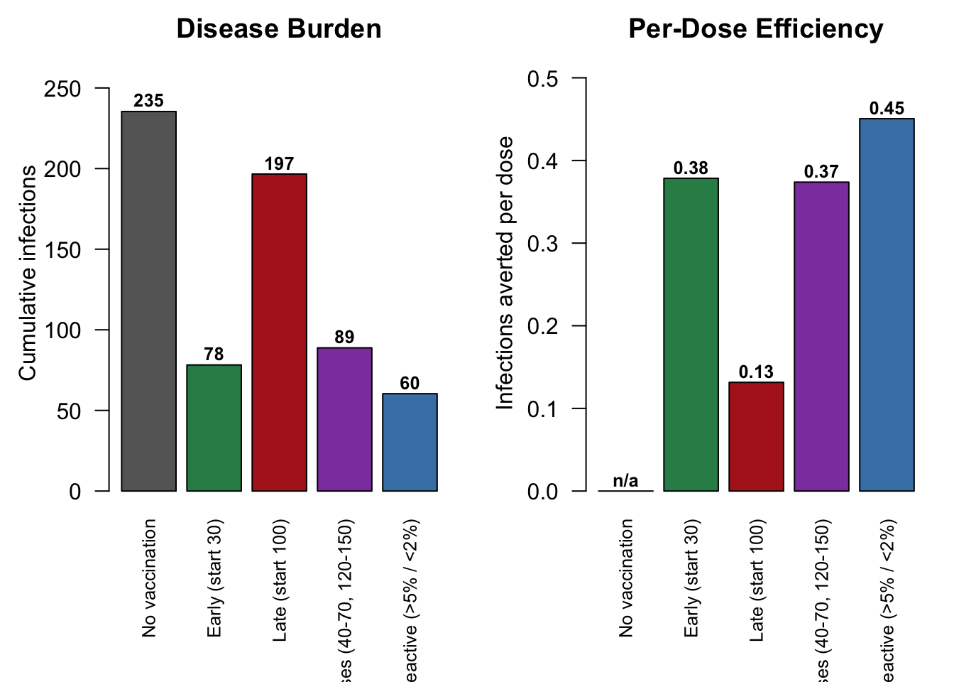
Endemic Comparison: Sustained Reactive Cycling
This is the headline phenomenon of the example. The top panel shows the SIRS dynamics with no intervention: a sustained endemic equilibrium that oscillates around the 5% activation threshold for the full simulation horizon. The bottom panel shows the same dynamics with the reactive program added: vaccination toggles on and off many times, suppressing each rising wave below the threshold and standing down when prevalence falls.
A single representative simulation is plotted because averaging across simulations smooths the binary on/off activity flag into a fractional value and hides the cycling.
sim_endemic_none <- mutate_epi(sim_endemic_none, prev = i.num / num)
sim_endemic_react <- mutate_epi(sim_endemic_react, prev = i.num / num)
df_n1 <- subset(as.data.frame(sim_endemic_none), sim == 1)
df_r1 <- subset(as.data.frame(sim_endemic_react), sim == 1)
ymax <- max(df_n1$i.num / df_n1$num, na.rm = TRUE) * 1.2

par(mfrow = c(2, 1), mar = c(3, 4, 2, 4), mgp = c(2.5, 1, 0))
plot(df_n1$time, df_n1$prev, type = "l", lwd = 2, col = "firebrick",
     xlab = "Time Step", ylab = "Prevalence (I / N)",
     main = "Endemic SIRS without Intervention (sim 1)",
     ylim = c(0, ymax))
abline(h = 0.05, lty = 2, col = "firebrick", lwd = 0.6)

plot(df_r1$time, df_r1$prev, type = "l", lwd = 2, col = "steelblue",
     xlab = "Time Step", ylab = "Prevalence (I / N)",
     main = "Endemic SIRS + Reactive Vaccination (sim 1)",
     ylim = c(0, ymax))
abline(h = 0.05, lty = 2, col = "firebrick")
abline(h = 0.02, lty = 2, col = "seagreen")
par(new = TRUE)
plot(df_r1$time, df_r1$vax.active, type = "s", lwd = 1.5,
     col = "gray40", axes = FALSE, xlab = "", ylab = "",
     ylim = c(0, 1.05))
axis(4)
mtext("Vaccination active (0/1)", side = 4, line = 2.5)
legend("topright",
       legend = c("Prevalence", "Activation 5%",
                  "Deactivation 2%", "Program active"),
       col = c("steelblue", "firebrick", "seagreen", "gray40"),
       lty = c(1, 2, 2, 1), lwd = c(2, 1, 1, 1.5), bty = "n",
       cex = 0.75)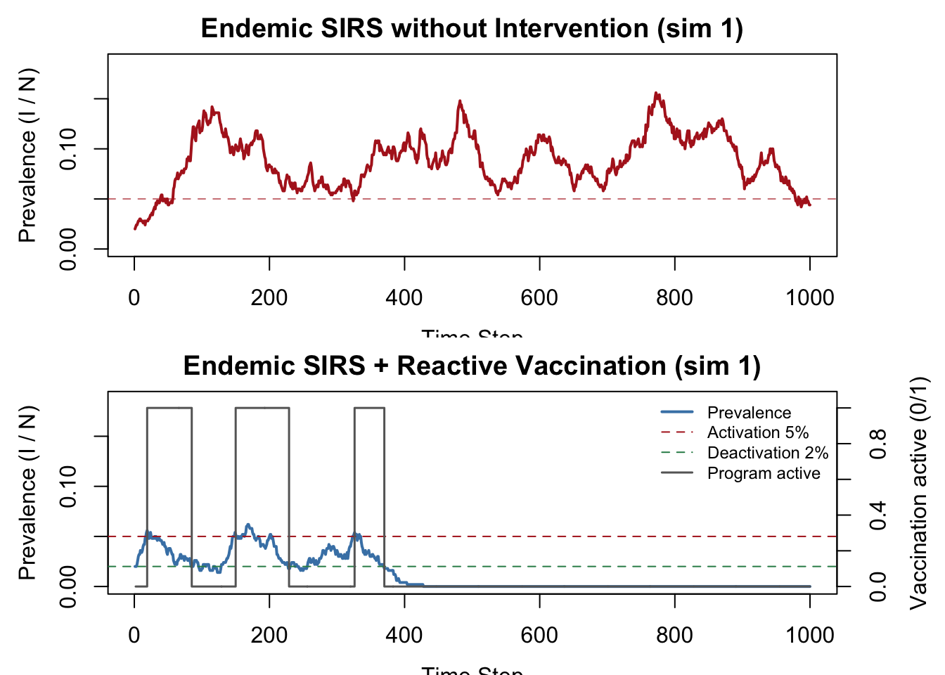
Summary Table
final_v <- sapply(sims, function(s) {
  df <- as.data.frame(s)
  round(mean(df$v.num[df$time == max(df$time)], na.rm = TRUE))
})
pct_averted <- ifelse(names(averted) == "none", "--",
                      paste0(round(averted / cum_inf["none"] * 100), "%"))
apd_str <- ifelse(is.na(avert_per_dose), "--",
                  sprintf("%.2f", avert_per_dose))

knitr::kable(data.frame(
  Scenario = labels,
  Cum_inf = round(cum_inf),
  Averted = ifelse(names(averted) == "none", 0, round(averted)),
  Pct_averted = pct_averted,
  Doses = round(total_vax),
  Averted_per_dose = apd_str,
  Vacc_immune_end = final_v,
  row.names = NULL
))| Scenario | Cum_inf | Averted | Pct_averted | Doses | Averted_per_dose | Vacc_immune_end |
|---|---|---|---|---|---|---|
| No vaccination | 258 | 0 | – | 0 | – | 0 |
| Early (start 30) | 70 | 188 | 73% | 422 | 0.44 | 387 |
| Late (start 100) | 133 | 125 | 49% | 358 | 0.35 | 323 |
| Pulses (40-70, 120-150) | 74 | 184 | 71% | 404 | 0.45 | 366 |
| Reactive (>5% / <2%) | 65 | 192 | 75% | 393 | 0.49 | 353 |
Timing Sensitivity Sweep
Sweeping the campaign start time from 0 to 200 traces a dose-response style curve for when to deploy. Below about timestep 60, the marginal benefit of a one-step delay is small; above that, the curve drops sharply as the campaign begins to miss the bulk of the epidemic.
sweep_starts <- seq(0, 200, by = 20)
sweep.df <- data.frame(
  .scenario.id = paste0("start_", sweep_starts),
  .at          = 0,
  vax.starts_1 = sweep_starts,
  vax.starts_2 = -1,
  vax.ends_1   = nsteps,
  vax.ends_2   = -1
)
sweep.list <- create_scenario_list(sweep.df)
sweep_cum <- numeric(length(sweep.list))
for (i in seq_along(sweep.list)) {
  s <- netsim(est, use_scenario(param_base, sweep.list[[i]]),
              init, control)
  df <- as.data.frame(s)
  sweep_cum[i] <- mean(tapply(df$si.flow, df$sim, sum, na.rm = TRUE))
}
sweep_pct <- 100 * (cum_inf["none"] - sweep_cum) / cum_inf["none"]

par(mfrow = c(1, 2), mar = c(3.5, 4, 2, 1), mgp = c(2.4, 1, 0))
plot(sweep_starts, sweep_cum, type = "b", pch = 19, lwd = 2,
     col = "steelblue", xlab = "Campaign start timestep",
     ylab = "Cumulative infections",
     main = "Burden vs. Start Time")
abline(h = cum_inf["none"], lty = 2, col = "gray50")
plot(sweep_starts, sweep_pct, type = "b", pch = 19, lwd = 2,
     col = "seagreen", xlab = "Campaign start timestep",
     ylab = "% infections averted",
     main = "Benefit by Start Time", ylim = c(0, 100))
Note
The sweep adds ~1 minute of runtime on a laptop (11 simulations at nsteps = 400, nsims = 5). The chunk is set with eval: false so the rendered page uses the figure baked in via freeze: auto. To run it yourself, set eval: true (or paste into your R session) — the included model.R runs it under if (interactive()).
Parameters
Disease
| Parameter | Description | Default |
|---|---|---|
inf.prob |
Per-act transmission probability | 0.10 |
act.rate |
Acts per partnership per timestep | 1 |
rec.rate |
Per-timestep recovery rate (mean infectious ~25) | 0.04 |
rs.rate |
R-to-S waning rate (0 = SIR; > 0 = SIRS) |
0 |
exog.inf.prob |
Per-S probability of exogenous infection per step | 0 |
Vaccination
| Parameter | Description | Default |
|---|---|---|
vax.rate |
Per-S vaccination probability per active timestep | 0.05 |
vax.efficacy |
All-or-nothing protection probability | 0.9 |
vax.wane |
V-to-S waning rate (0 = permanent vaccine immunity) |
0 |
Schedule
| Parameter | Description | Disabled |
|---|---|---|
vax.starts |
Vector of window start timesteps | -1 |
vax.ends |
Vector of window end timesteps | -1 |
vax.prev.on |
Reactive activation threshold | -1 |
vax.prev.off |
Reactive deactivation threshold | -1 |
Reactive mode is selected when vax.prev.on > 0. Otherwise the module uses the windowed schedule.
Network
| Parameter | Description | Default |
|---|---|---|
| Population size | Number of nodes | 500 |
| Target edges | Mean concurrent partnerships | 375 (mean degree = 1.5) |
| Partnership duration | Mean edge duration (timesteps) | 60 |
Module Execution Order
resim_nets -> summary_nets -> infection -> recovery -> vaccinate -> nwupdate -> prevalenceEpiModel’s default pipeline. Our three custom modules (infect, recov, vaccinate) replace the corresponding built-in slots; the rest are EpiModel built-ins. The built-in prevalence.net runs last and fills in s.num, i.num, and num from the updated status vector.
Next Steps
- Combine timing with a leaky vaccine by porting the schedule pattern to the leaky-vaccine module — see SEIRS with Leaky Vaccination.
- Phase a testing or treatment intervention instead of vaccination. The same windowed and reactive logic can wrap any rate parameter — see Test and Treat Intervention.
- Time-vary the disease parameters themselves, e.g. a seasonal
inf.prob, by applying the sameat-dependent gate inside the infection module. - Combine windowed and reactive logic: a planned campaign that can be extended if prevalence remains above a threshold.
- Layer onto a model with vital dynamics so vaccination must keep up with the inflow of new susceptibles — see SEIR with AON Vaccination.