flowchart LR
    S((S)) -->|"infection"| Inc["Incubating"]
    Inc -->|"~4 wk"| Pri["Primary"]
    Pri -->|"~9 wk"| Sec["Secondary"]
    Sec -->|"~17 wk"| EL["Early Latent"]
    EL -->|"~22 wk"| LL["Late Latent"]
    LL -->|"~29 yr"| Ter["Tertiary"]

    Pri -.->|"symptomatic trt"| S
    Sec -.->|"symptomatic trt"| S
    Ter -.->|"symptomatic trt"| S
    Inc -.->|"screening"| S
    EL -.->|"screening"| S
    LL -.->|"screening"| S

    style Inc fill:#95a5a6,color:#fff
    style Pri fill:#e74c3c,color:#fff
    style Sec fill:#e74c3c,color:#fff
    style EL fill:#f39c12,color:#fff
    style LL fill:#95a5a6,color:#fff
    style Ter fill:#95a5a6,color:#fff
Syphilis Progression Model
multi-stage
syphilis
diagnosis
treatment
advanced
Models multi-stage syphilis transmission, progression, diagnosis, and treatment with stage-dependent infectiousness and screening-driven recovery.
Overview
This example models the transmission, multi-stage progression, diagnosis, and treatment of syphilis using EpiModel’s network-based framework. It extends the basic SI model by adding multiple disease compartments representing the natural history of syphilis, plus a treatment and screening module that allows infected individuals to recover back to the susceptible state. The result is an SIS-type model — individuals who recover return to the susceptible pool and can be reinfected — but with six intermediate disease stages governing infectiousness, symptoms, and treatment eligibility.
Syphilis progresses through incubation, primary, secondary, early latent, late latent, and tertiary stages. Stage-specific transmission probabilities are aligned with CDC’s clinical framing: sexual transmission occurs primarily through contact with mucocutaneous syphilitic lesions (CDC, About Syphilis; CDC STI Treatment Guidelines, Syphilis). The chancre (primary), mucous patches and condylomata lata (secondary), and clinical relapses during the first year (early latent) carry transmissibility; the pre-chancre incubation period, late latent, and tertiary stages do not. CDC’s surveillance definition of “infectious syphilis” — primary, secondary, and early non-primary non-secondary (early latent) — maps directly to the stages with positive per-act transmission probability in this model. Only a fraction of primary and secondary infections produce recognizable symptoms, so most cases are clinically silent and can only be detected through population-level screening.
This is a simplified pedagogical model intended to demonstrate how to build a multi-stage disease model in EpiModel with stage-dependent transmission, symptom-driven diagnosis, and population-level screening. The two-scenario comparison — annual screening versus no screening — highlights how routine screening can dramatically reduce the latent reservoir of untreated syphilis even though recovered individuals face ongoing reinfection risk.
TipDownload the Model Scripts
You can download the standalone scripts to run this example outside of this tutorial:
- model.R — main simulation script
- module-fx.R — custom module functions
Model Structure
Disease Compartments
Syphilis progresses through six stages, each tracked by the syph.stage nodal attribute. Susceptible individuals have syph.stage = NA and status = "s".
| Stage | syph.stage |
Per-act transmission | Symptomatic | Duration (mean) |
|---|---|---|---|---|
| Incubating | "incubating" |
inf.prob.incubating (default 0; pre-chancre) |
No | ~4 weeks |
| Primary | "primary" |
inf.prob.early (0.18; chancre) |
Possible | ~9 weeks |
| Secondary | "secondary" |
inf.prob.early (0.18; mucous patches, condylomata) |
Possible | ~17 weeks |
| Early Latent | "early_latent" |
inf.prob.latent (0.09; clinical relapses) |
No | ~22 weeks |
| Late Latent | "late_latent" |
0 (hard-coded) | No | ~29 years |
| Tertiary | "tertiary" |
0 (hard-coded) | Yes | Terminal |
Flow Diagram
The diagram below shows disease progression (solid arrows) and treatment or screening recovery pathways (dashed arrows) back to susceptible. Red nodes are infectious at the higher rate (primary and secondary, with mucocutaneous lesions present); orange is infectious at the reduced early-latent rate; gray nodes are non-transmitting (incubating, late latent, tertiary).
Transmission
Transmission probability depends on the infector’s stage:
- Primary and secondary (
inf.prob.early, default 0.18 per act): mucocutaneous lesions (chancre, mucous patches, condylomata lata) present; this is the conventional route of sexual transmission. - Early latent (
inf.prob.latent, default 0.09 per act): roughly half the early-stage rate, representing residual transmission during clinical relapses of secondary lesions within the first year of infection. Together with primary and secondary, this matches CDC’s “infectious syphilis” surveillance definition. - Incubating (
inf.prob.incubating, default 0): the chancre has not yet appeared, so the mucocutaneous-lesion transmission route is by definition absent. The default value sets sexual transmission to zero during incubation; users can set it positive as a sensitivity analysis on pre-chancre transmission. - Late latent and tertiary: hard-coded to zero (no sexual transmission).
The per-partnership transmission rate applies the standard EpiModel formula: finalProb = 1 - (1 - transProb)^actRate. References: CDC About Syphilis; CDC STI Treatment Guidelines, Syphilis (2021); Garnett GP et al. (1997), The natural history of syphilis, Sex Transm Dis 24(4):185-200.
Treatment Pathways
There are two routes to treatment:
- Symptomatic diagnosis — Individuals who develop symptoms during the primary or secondary stage may seek treatment (probability
early.trtper timestep). Tertiary-stage patients, who are always symptomatic, may receive treatment at ratelate.trt. - Population screening — Asymptomatic infected individuals may be detected through routine screening (probability
scr.rateper timestep).
Recovery times after treatment initiation vary by stage: primary and secondary recover in 1 week, screening-detected cases in 2 weeks, and tertiary in 3 weeks. Upon recovery, individuals return to the susceptible state.
Setup
We begin by loading EpiModel and setting the simulation parameters. The interactive() values below are designed for a full analysis; reduce them for faster test runs.
library(EpiModel)

nsims <- 5
ncores <- 5
nsteps <- 500
Custom Modules
This model uses three custom modules that replace EpiModel’s built-in infection and recovery functions: an infection module with stage-dependent transmission, a progression module that moves individuals through six syphilis stages, and a treatment and screening module that handles both symptomatic diagnosis and population-level screening.
Infection Module
The infection module extends EpiModel’s standard infection logic with two key additions: initialization of all custom attributes at the first timestep, and stage-dependent transmission probabilities. All syphilis-related nodal attributes — stage, symptoms, treatment status, and timing variables — are set up at at == 2 (EpiModel reserves timestep 1 for network initialization).
After initialization, the module identifies discordant partnerships (one susceptible, one infected partner) and computes transmission probability based on the infector’s current syphilis stage. Newly infected individuals enter the incubating stage.
infect <- function(dat, at) {

  ## Attributes ##
  active <- get_attr(dat, "active")
  status <- get_attr(dat, "status")

  ## Initialize all custom attributes at the first timestep ##
  if (at == 2) {
    dat <- set_attr(dat, "syph.stage",
1                    ifelse(status == "i", "incubating", NA))
    dat <- set_attr(dat, "syph.symp", rep(0, length(active)))
    dat <- set_attr(dat, "infTime", ifelse(status == "i", 1, NA))
    dat <- set_attr(dat, "priTime", rep(NA, length(active)))
    dat <- set_attr(dat, "secTime", rep(NA, length(active)))
    dat <- set_attr(dat, "elTime", rep(NA, length(active)))
    dat <- set_attr(dat, "llTime", rep(NA, length(active)))
    dat <- set_attr(dat, "terTime", rep(NA, length(active)))
    dat <- set_attr(dat, "syph.dur", rep(NA, length(active)))
    dat <- set_attr(dat, "syph2.dur", rep(NA, length(active)))
    dat <- set_attr(dat, "syph3.dur", rep(NA, length(active)))
    dat <- set_attr(dat, "syph4.dur", rep(NA, length(active)))
    dat <- set_attr(dat, "syph5.dur", rep(NA, length(active)))
    dat <- set_attr(dat, "syph6.dur", rep(NA, length(active)))
    dat <- set_attr(dat, "syph.trt", rep(NA, length(active)))
    dat <- set_attr(dat, "syph.scr", rep(0, length(active)))
    dat <- set_attr(dat, "trtTime", rep(NA, length(active)))
    dat <- set_attr(dat, "scrTime", rep(NA, length(active)))
  }

  syph.stage <- get_attr(dat, "syph.stage")
  infTime <- get_attr(dat, "infTime")

  ## Parameters ##
  inf.prob.incubating <- get_param(dat, "inf.prob.incubating")
  inf.prob.early <- get_param(dat, "inf.prob.early")
  inf.prob.latent <- get_param(dat, "inf.prob.latent")
  act.rate <- get_param(dat, "act.rate")

  ## Find infected nodes ##
  idsInf <- which(active == 1 & status == "i")
  nActive <- sum(active == 1)
  nElig <- length(idsInf)

  ## Initialize default incidence at 0 ##
  nInf <- 0

  ## If any infected nodes, proceed with transmission ##
  if (nElig > 0 && nElig < nActive) {
2    del <- discord_edgelist(dat, at)

    if (!(is.null(del))) {
3      stage <- syph.stage[del$inf]
      del$transProb <- ifelse(
        stage %in% c("primary", "secondary"), inf.prob.early,
        ifelse(stage == "early_latent", inf.prob.latent,
        ifelse(stage == "incubating", inf.prob.incubating, 0)))

      del$actRate <- act.rate
4      del$finalProb <- 1 - (1 - del$transProb)^del$actRate

      transmit <- rbinom(nrow(del), 1, del$finalProb)
      del <- del[which(transmit == 1), ]
      idsNewInf <- unique(del$sus)
      nInf <- length(idsNewInf)

      if (nInf > 0) {
        syph.stage[idsNewInf] <- "incubating"
        status[idsNewInf] <- "i"
        infTime[idsNewInf] <- at
      }
    }
  }

  ## Save updated attributes ##
  dat <- set_attr(dat, "status", status)
  dat <- set_attr(dat, "syph.stage", syph.stage)
  dat <- set_attr(dat, "infTime", infTime)

  ## Save summary statistics ##
  dat <- set_epi(dat, "si.flow", at, nInf)
  syph.dur <- get_attr(dat, "syph.dur")
  syph.dur <- ifelse(syph.stage == "incubating", (at - infTime), syph.dur)
  dat <- set_attr(dat, "syph.dur", syph.dur)
5  dat <- set_epi(dat, "syph.dur", at, mean(syph.dur, na.rm = TRUE))

  return(dat)
}- 1
-
At timestep 2, all custom attributes are initialized: initially infected nodes start in the
"incubating"stage while susceptible nodes getNA. - 2
-
discord_edgelist()identifies partnerships where one node is susceptible and the other is infected — these are the only partnerships where transmission can occur. - 3
-
Transmission probability is stage-dependent: primary/secondary use
inf.prob.early(mucocutaneous lesions present), early latent usesinf.prob.latent(clinical relapses), incubating usesinf.prob.incubating(default 0; pre-chancre), and late latent/tertiary are zero. - 4
-
The final per-partnership probability accounts for multiple acts:
1 - (1 - p)^actsconverts per-act probability to per-partnership probability over the timestep. - 5
- Mean duration in the incubating stage is tracked as an epidemiological summary statistic across all currently incubating individuals.
Progression Module
The progression module simulates transitions between the six syphilis stages. Each transition is a stochastic Bernoulli process with a constant hazard rate, so time spent in each compartment follows a geometric distribution. A minimum one-timestep delay is enforced before any transition (for example, infTime < at for incubating-to-primary) to prevent instant progression.
Symptomatic status is assigned stochastically at entry to the primary and secondary stages with probabilities pri.sym and sec.sym. Most infections remain asymptomatic — approximately 80% of primary and 89% of secondary cases are clinically silent. Tertiary-stage individuals are always symptomatic.
progress <- function(dat, at) {

  ## Attributes ##
  active <- get_attr(dat, "active")
  syph.stage <- get_attr(dat, "syph.stage")
  syph.symp <- get_attr(dat, "syph.symp")
  infTime <- get_attr(dat, "infTime")
  priTime <- get_attr(dat, "priTime")
  secTime <- get_attr(dat, "secTime")
  elTime <- get_attr(dat, "elTime")
  llTime <- get_attr(dat, "llTime")
  terTime <- get_attr(dat, "terTime")

  ## Parameters of stage transition ##
  ipr.rate <- get_param(dat, "ipr.rate")
  prse.rate <- get_param(dat, "prse.rate")
  seel.rate <- get_param(dat, "seel.rate")
  elll.rate <- get_param(dat, "elll.rate")
  llter.rate <- get_param(dat, "llter.rate")

  ## Parameters of symptomatic progression ##
  pri.sym <- get_param(dat, "pri.sym")
  sec.sym <- get_param(dat, "sec.sym")

  ## Incubation to primary stage ##
  nPrim <- 0
  idsEligPri <- which(active == 1 & syph.stage == "incubating" &
1                        infTime < at)
  nEligPri <- length(idsEligPri)

  if (nEligPri > 0) {
    vecPri <- which(rbinom(nEligPri, 1, ipr.rate) == 1)
    if (length(vecPri) > 0) {
      idsPri <- idsEligPri[vecPri]
      nPrim  <- length(idsPri)
      syph.stage[idsPri] <- "primary"
      priTime[idsPri] <- at
      syph.symp[idsPri] <- sample(0:1, size = length(vecPri),
                                  prob = c(1 - pri.sym, pri.sym),
2                                  replace = TRUE)
    }
  }

  syph2.dur <- get_attr(dat, "syph2.dur")
  dat <- set_attr(dat, "syph2.dur",
                  ifelse(syph.stage == "primary", (at - priTime), syph2.dur))

  ## Primary to secondary stage ##
  nSec <- 0
  idsEligSec <- which(active == 1 & syph.stage == "primary" & priTime < at)
  nEligSec <- length(idsEligSec)

  if (nEligSec > 0) {
    vecSec <- which(rbinom(nEligSec, 1, prse.rate) == 1)
    if (length(vecSec) > 0) {
      idsSec <- idsEligSec[vecSec]
      nSec <- length(idsSec)
      syph.stage[idsSec] <- "secondary"
      syph.symp[idsSec] <- 0
      secTime[idsSec] <- at
      syph.symp[idsSec] <- sample(0:1, size = length(vecSec),
                                  prob = c(1 - sec.sym, sec.sym),
                                  replace = TRUE)
    }
  }

  syph3.dur <- get_attr(dat, "syph3.dur")
  dat <- set_attr(dat, "syph3.dur",
                  ifelse(syph.stage == "secondary", (at - secTime), syph3.dur))

  ## Secondary to early latent ##
  nEarL <- 0
  idsEligLat <- which(active == 1 & syph.stage == "secondary" & secTime < at)
  nEligLat <- length(idsEligLat)

  if (nEligLat > 0) {
    vecLat <- which(rbinom(nEligLat, 1, seel.rate) == 1)
    if (length(vecLat) > 0) {
      idsLat <- idsEligLat[vecLat]
      nEarL <- length(idsLat)
      syph.stage[idsLat] <- "early_latent"
3      syph.symp[idsLat] <- 0
      elTime[idsLat] <- at
    }
  }

  syph4.dur <- get_attr(dat, "syph4.dur")
  dat <- set_attr(dat, "syph4.dur",
                  ifelse(syph.stage == "early_latent",
                         (at - elTime), syph4.dur))

  ## Early latent to late latent ##
  nLaL <- 0
  idsEligLaL <- which(active == 1 & syph.stage == "early_latent" & elTime < at)
  nEligLaL <- length(idsEligLaL)

  if (nEligLaL > 0) {
    vecLal <- which(rbinom(nEligLaL, 1, elll.rate) == 1)
    if (length(vecLal) > 0) {
      idsLal <- idsEligLaL[vecLal]
      nLaL <- length(idsLal)
      syph.stage[idsLal] <- "late_latent"
      syph.symp[idsLal] <- 0
      llTime[idsLal] <- at
    }
  }

  syph5.dur <- get_attr(dat, "syph5.dur")
  llTime <- get_attr(dat, "llTime")
  dat <- set_attr(dat, "syph5.dur",
                  ifelse(syph.stage == "late_latent",
                         (at - llTime), syph5.dur))

  ## Late latent to tertiary ##
  nTer <- 0
  idsEligTer <- which(active == 1 & syph.stage == "late_latent" & llTime < at)
  nEligTer <- length(idsEligTer)

  if (nEligTer > 0) {
    vecTer <- which(rbinom(nEligTer, 1, llter.rate) == 1)
    if (length(vecTer) > 0) {
      idsTer <- idsEligTer[vecTer]
      nTer <- length(idsTer)
      syph.stage[idsTer] <- "tertiary"
4      syph.symp[idsTer] <- 1
      terTime[idsTer] <- at
    }
  }

  syph6.dur <- get_attr(dat, "syph6.dur")
  dat <- set_attr(dat, "syph6.dur",
                  ifelse(syph.stage == "tertiary",
                         (at - terTime), syph6.dur))

  ## Save updated attributes ##
  dat <- set_attr(dat, "syph.stage", syph.stage)
  dat <- set_attr(dat, "syph.symp", syph.symp)
  dat <- set_attr(dat, "priTime", priTime)
  dat <- set_attr(dat, "secTime", secTime)
  dat <- set_attr(dat, "elTime", elTime)
  dat <- set_attr(dat, "llTime", llTime)
  dat <- set_attr(dat, "terTime", terTime)

  ## Save summary statistics ##
  dat <- set_epi(dat, "ipr.flow", at, nPrim)
  dat <- set_epi(dat, "prse.flow", at, nSec)
  dat <- set_epi(dat, "seel.flow", at, nEarL)
  dat <- set_epi(dat, "elll.flow", at, nLaL)
  dat <- set_epi(dat, "llter.flow", at, nTer)

  dat <- set_epi(dat, "inc.num", at,
                 sum(active == 1 & syph.stage == "incubating", na.rm = TRUE))
  dat <- set_epi(dat, "pr.num", at,
                 sum(active == 1 & syph.stage == "primary", na.rm = TRUE))
  dat <- set_epi(dat, "se.num", at,
                 sum(active == 1 & syph.stage == "secondary", na.rm = TRUE))
  dat <- set_epi(dat, "el.num", at,
                 sum(active == 1 & syph.stage == "early_latent", na.rm = TRUE))
  dat <- set_epi(dat, "ll.num", at,
                 sum(active == 1 & syph.stage == "late_latent", na.rm = TRUE))
  dat <- set_epi(dat, "ter.num", at,
                 sum(active == 1 & syph.stage == "tertiary", na.rm = TRUE))
5  dat <- set_epi(dat, "sym.num", at,
                 sum(active == 1 & syph.symp == 1, na.rm = TRUE))

  dat <- set_epi(dat, "syph2.dur", at, mean(syph2.dur, na.rm = TRUE))
  dat <- set_epi(dat, "syph3.dur", at, mean(syph3.dur, na.rm = TRUE))
  dat <- set_epi(dat, "syph4.dur", at, mean(syph4.dur, na.rm = TRUE))
  dat <- set_epi(dat, "syph5.dur", at, mean(syph5.dur, na.rm = TRUE))
  dat <- set_epi(dat, "syph6.dur", at, mean(syph6.dur, na.rm = TRUE))

  return(dat)
}- 1
-
The
infTime < atcondition enforces a minimum one-timestep delay before any stage transition, preventing individuals from progressing through multiple stages in a single timestep. - 2
-
Symptomatic status is assigned stochastically at primary stage entry:
pri.sym = 0.205means roughly 20% of primary infections produce recognizable symptoms. - 3
- Latent stages are always asymptomatic — symptoms are reset to 0 upon entering early latent, making these cases invisible to symptomatic diagnosis.
- 4
-
Tertiary syphilis is always symptomatic (
syph.symp = 1), unlike earlier stages where symptom status is probabilistic. - 5
-
Summary statistics track the count in each stage and the number of symptomatic individuals at every timestep, which are stored via
set_epi()for post-simulation analysis.
Treatment and Screening Module
The treatment and screening module (tnt) handles all recovery pathways. It is organized into four sequential phases: symptomatic treatment initiation, symptomatic treatment recovery, screening of the asymptomatic infected population, and screening-detected recovery.
Symptomatic patients in the primary or secondary stage may begin treatment at rate early.trt per timestep, while tertiary patients use rate late.trt. Recovery occurs after a stage-dependent delay (1 week for early stages, 3 weeks for tertiary). Screening operates independently: asymptomatic infected individuals are tested at rate scr.rate, and those detected recover after a 2-week delay. Upon recovery from either pathway, individuals return to the susceptible pool.
tnt <- function(dat, at) {

  ## Attributes ##
  active <- get_attr(dat, "active")
  status <- get_attr(dat, "status")
  syph.stage <- get_attr(dat, "syph.stage")
  syph.symp <- get_attr(dat, "syph.symp")
  syph.trt <- get_attr(dat, "syph.trt")
  syph.scr <- get_attr(dat, "syph.scr")
  trtTime <- get_attr(dat, "trtTime")
  scrTime <- get_attr(dat, "scrTime")

  ## Parameters ##
  early.trt <- get_param(dat, "early.trt")
  late.trt <- get_param(dat, "late.trt")
  scr.rate <- get_param(dat, "scr.rate")

  # --- Symptomatic treatment initiation ---

  ## Primary symptomatic patients receiving treatment ##
  priTime <- get_attr(dat, "priTime")
  idsPriTrt <- which(active == 1 & syph.stage == "primary" &
                       syph.symp == 1 & is.na(syph.trt) &
1                       priTime < at)
  if (length(idsPriTrt) > 0) {
    vecPriTrt <- which(rbinom(length(idsPriTrt), 1, early.trt) == 1)
    if (length(vecPriTrt) > 0) {
      idsPriTrt <- idsPriTrt[vecPriTrt]
      syph.trt[idsPriTrt] <- 1
      trtTime[idsPriTrt] <- at
    }
  }

  ## Secondary symptomatic patients receiving treatment ##
  secTime <- get_attr(dat, "secTime")
  idsSecTrt <- which(active == 1 & syph.stage == "secondary" &
                       syph.symp == 1 & is.na(syph.trt) &
                       secTime < at)
  if (length(idsSecTrt) > 0) {
    vecSecTrt <- which(rbinom(length(idsSecTrt), 1, early.trt) == 1)
    if (length(vecSecTrt) > 0) {
      idsSecTrt <- idsSecTrt[vecSecTrt]
      syph.trt[idsSecTrt] <- 1
      trtTime[idsSecTrt] <- at
    }
  }

  ## Tertiary symptomatic patients receiving treatment ##
  terTime <- get_attr(dat, "terTime")
  idsTerTrt <- which(active == 1 & syph.stage == "tertiary" &
                       syph.symp == 1 & is.na(syph.trt) &
                       terTime < at)
  if (length(idsTerTrt) > 0) {
    vecTerTrt <- which(rbinom(length(idsTerTrt), 1, late.trt) == 1)
    if (length(vecTerTrt) > 0) {
      idsTerTrt <- idsTerTrt[vecTerTrt]
      syph.trt[idsTerTrt] <- 1
      trtTime[idsTerTrt] <- at
    }
  }

  # --- Symptomatic treatment recovery ---

  ## Recover 1 week after treatment (primary) ##
  idsPriRec <- which(active == 1 & syph.stage == "primary" &
2                       syph.trt == 1 & trtTime <= at - 1)
  if (length(idsPriRec) > 0) {
    status[idsPriRec] <- "s"
    syph.stage[idsPriRec] <- NA
    syph.trt[idsPriRec] <- NA
    syph.symp[idsPriRec] <- 0
  }

  ## Recover 1 week after treatment (secondary) ##
  idsSecRec <- which(active == 1 & syph.stage == "secondary" &
                       syph.trt == 1 & trtTime <= at - 1)
  if (length(idsSecRec) > 0) {
    status[idsSecRec] <- "s"
    syph.stage[idsSecRec] <- NA
    syph.trt[idsSecRec] <- NA
    syph.symp[idsSecRec] <- 0
  }

  ## Recover 3 weeks after treatment (tertiary) ##
  idsTerRec <- which(active == 1 & syph.stage == "tertiary" &
3                       syph.trt == 1 & trtTime <= at - 3)
  if (length(idsTerRec) > 0) {
    status[idsTerRec] <- "s"
    syph.stage[idsTerRec] <- NA
    syph.trt[idsTerRec] <- NA
    syph.symp[idsTerRec] <- 0
  }

  # --- Screening of asymptomatic infected population ---

  nScr <- 0
  idsEligScr <- which(active == 1 & status == "i" &
4                        syph.symp == 0 & is.na(syph.trt))
  nEligScr <- length(idsEligScr)

  if (nEligScr > 0) {
    vecScr <- which(rbinom(nEligScr, 1, scr.rate) == 1)
    if (length(vecScr) > 0) {
      idsScr <- idsEligScr[vecScr]
      nScr <- length(idsScr)
      syph.scr[idsScr] <- 1
      syph.trt[idsScr] <- 1
      trtTime[idsScr] <- at
      scrTime[idsScr] <- at
    }
  }

  # --- Screening-detected recovery ---

  idsRecScr <- which(active == 1 &
                       syph.stage %in% c("incubating", "primary",
                                         "secondary", "early_latent",
                                         "late_latent") &
                       syph.trt == 1 & trtTime < at - 1)
  if (length(idsRecScr) > 0) {
    status[idsRecScr] <- "s"
    syph.stage[idsRecScr] <- NA
    syph.trt[idsRecScr] <- NA
    syph.symp[idsRecScr] <- 0
  }

  ## Count total recoveries this timestep ##
  nRec <- length(idsPriRec) + length(idsSecRec) +
    length(idsTerRec) + length(idsRecScr)

  ## Save all modified attributes ##
  dat <- set_attr(dat, "status", status)
  dat <- set_attr(dat, "syph.stage", syph.stage)
  dat <- set_attr(dat, "syph.symp", syph.symp)
  dat <- set_attr(dat, "syph.trt", syph.trt)
  dat <- set_attr(dat, "syph.scr", syph.scr)
  dat <- set_attr(dat, "trtTime", trtTime)
  dat <- set_attr(dat, "scrTime", scrTime)

  ## Save summary statistics ##
  dat <- set_epi(dat, "rec.flow", at, nRec)
  dat <- set_epi(dat, "scr.flow", at, nScr)
  dat <- set_epi(dat, "scr.num", at,
                 sum(active == 1 & syph.scr == 1, na.rm = TRUE))
5  dat <- set_epi(dat, "trt.num", at,
                 sum(active == 1 & syph.trt == 1, na.rm = TRUE))

  return(dat)
}- 1
-
Treatment eligibility requires four conditions: the individual must be active, in the correct stage, symptomatic (
syph.symp == 1), not already on treatment (is.na(syph.trt)), and past the minimum delay since entering the stage. - 2
-
Primary and secondary patients recover 1 week after treatment initiation (
trtTime <= at - 1), at which point all disease attributes are reset to susceptible values. - 3
-
Tertiary patients require a longer 3-week treatment course (
trtTime <= at - 3) before recovery, reflecting the greater clinical severity. - 4
- Screening targets only asymptomatic infected individuals who are not already on treatment — symptomatic cases are handled by the treatment pathway above.
- 5
-
Summary statistics track total recoveries (
rec.flow), new screenings (scr.flow), cumulative screened (scr.num), and currently on treatment (trt.num) at each timestep.
Network Model
Network Initialization
We initialize a 1,000-node network representing a sexual contact network. The formation model uses edges and isolates terms to control both the mean degree and the proportion of individuals with no current partner.
n <- 1000
nw <- network_initialize(n)
Formation and Dissolution
The target statistics specify 300 edges (mean degree 0.6) and 480 isolates (48% of the population with no current partner at any given time). This creates a network where roughly half the population is not sexually active at any point. Partnerships last an average of 10 weeks.
formation <- ~edges + isolates
target.stats <- c(300, 480)

coef.diss <- dissolution_coefs(dissolution = ~offset(edges), duration = 10)
coef.diss
Dissolution Coefficients
=======================
Dissolution Model: ~offset(edges)
Target Statistics: 10
Crude Coefficient: 2.197225
Mortality/Exit Rate: 0
Adjusted Coefficient: 2.197225Network Estimation
The network model is fit using netest(), which estimates the ERGM coefficients needed to produce the target network statistics under the specified dissolution model.
est <- netest(nw, formation, target.stats, coef.diss)Network Diagnostics
After estimation, we run diagnostics to verify that the simulated dynamic network produces edge counts and degree distributions consistent with the target statistics.
dx <- netdx(est, nsims = nsims, ncores = ncores, nsteps = nsteps,
            nwstats.formula = ~edges + isolates + degree(0:3))
Network Diagnostics
-----------------------
- Simulating 5 networks
- Calculating formation statisticsprint(dx)EpiModel Network Diagnostics
=======================
Diagnostic Method: Dynamic
Simulations: 5
Time Steps per Sim: 500
Formation Diagnostics
-----------------------
Target Sim Mean Pct Diff Sim SE Z Score SD(Sim Means) SD(Statistic)
edges 300 286.977 -4.341 0.875 -14.889 1.157 13.397
isolates 480 501.764 4.534 1.245 17.477 1.272 20.005
degree0 NA 501.764 NA 1.245 NA 1.272 20.005
degree1 NA 429.288 NA 0.954 NA 1.851 17.280
degree2 NA 62.626 NA 0.474 NA 1.251 8.442
degree3 NA 5.912 NA 0.121 NA 0.321 2.498
Duration Diagnostics
-----------------------
Target Sim Mean Pct Diff Sim SE Z Score SD(Sim Means) SD(Statistic)
edges 10 9.964 -0.362 0.046 -0.788 0.098 0.571
Dissolution Diagnostics
-----------------------
Target Sim Mean Pct Diff Sim SE Z Score SD(Sim Means) SD(Statistic)
edges 0.1 0.1 -0.008 0 -0.023 0 0.018plot(dx)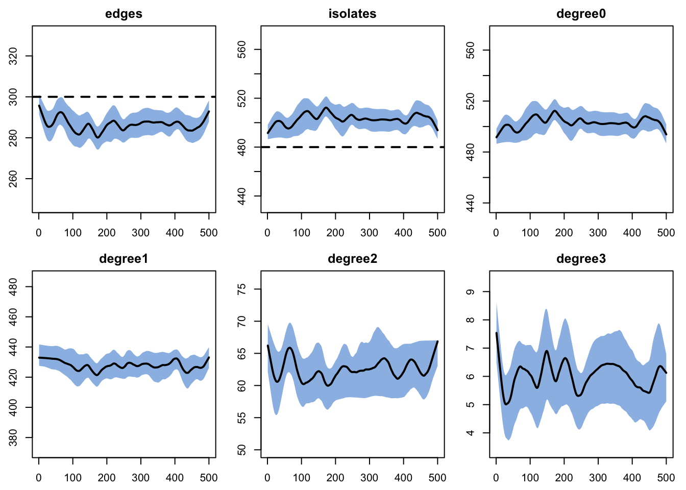
Note
The diagnostics may show values roughly 5% off from the targets. This is due to the edges dissolution approximation used for quickly fitting the TERGM in the context of a short overall partnership duration (10 weeks). There are various ways to handle this (see ?netest) but we ignore this minor discrepancy for the current purposes.
Epidemic Simulation
Initial Conditions and Parameters
We set up two scenarios to compare the impact of population screening. Both use identical disease parameters; the only difference is whether scr.rate is set to 1/52 (annual screening) or 0 (no screening).
init <- init.net(i.num = 10)Scenario 1: With Annual Screening
The first scenario includes population-level screening at a rate of approximately once per year (scr.rate = 1/52), allowing asymptomatic cases to be detected and treated.
param_scr <- param.net(
  inf.prob.incubating = 0,
  inf.prob.early = 0.18,
  inf.prob.latent = 0.09,
  act.rate = 2,
  ipr.rate = 1 / 4,
  prse.rate = 1 / 9,
  seel.rate = 1 / 17,
  elll.rate = 1 / 22,
  llter.rate = 1 / 1508,
  pri.sym = 0.205,
  sec.sym = 0.106,
  early.trt = 0.8,
  late.trt = 1.0,
  scr.rate = 1 / 52
)
Scenario 2: No Screening
The second scenario disables screening entirely. Without screening, only the roughly 20% of primary and 11% of secondary infections that produce recognizable symptoms can ever be detected and treated. The vast majority of infections progress silently through the latent stages, creating a large untreatable reservoir.
param_noscr <- param.net(
  inf.prob.incubating = 0,
  inf.prob.early = 0.18,
  inf.prob.latent = 0.09,
  act.rate = 2,
  ipr.rate = 1 / 4,
  prse.rate = 1 / 9,
  seel.rate = 1 / 17,
  elll.rate = 1 / 22,
  llter.rate = 1 / 1508,
  pri.sym = 0.205,
  sec.sym = 0.106,
  early.trt = 0.8,
  late.trt = 1.0,
  scr.rate = 0
)
Control Settings and Simulation
The control object specifies a fully custom module set (type = NULL) with explicit module execution order. Because this model has no vital dynamics (closed population), resimulate.network is set to FALSE.
control <- control.net(
  type = NULL,
  nsteps = nsteps,
  nsims = nsims,
  ncores = ncores,
  infection.FUN = infect,
  progress.FUN = progress,
  tnt.FUN = tnt,
  resimulate.network = FALSE,
  module.order = c("resim_nets.FUN",
                   "infection.FUN",
                   "progress.FUN",
                   "tnt.FUN",
                   "prevalence.FUN")
)
sim_scr <- netsim(est, param_scr, init, control)
print(sim_scr)EpiModel Simulation
=======================
Model class: netsim
Simulation Summary
-----------------------
Model type:
No. simulations: 5
No. time steps: 500
No. NW groups: 1
Fixed Parameters
---------------------------
act.rate = 2
inf.prob.incubating = 0
inf.prob.early = 0.18
inf.prob.latent = 0.09
ipr.rate = 0.25
prse.rate = 0.1111111
seel.rate = 0.05882353
elll.rate = 0.04545455
llter.rate = 0.00066313
pri.sym = 0.205
sec.sym = 0.106
early.trt = 0.8
late.trt = 1
scr.rate = 0.01923077
groups = 1
Model Functions
-----------------------
initialize.FUN
resim_nets.FUN
summary_nets.FUN
infection.FUN
nwupdate.FUN
prevalence.FUN
verbose.FUN
progress.FUN
tnt.FUN
Model Output
-----------------------
Variables: s.num i.num num si.flow syph.dur ipr.flow
prse.flow seel.flow elll.flow llter.flow inc.num pr.num
se.num el.num ll.num ter.num sym.num syph2.dur syph3.dur
syph4.dur syph5.dur syph6.dur rec.flow scr.flow scr.num
trt.num
Networks: sim1 ... sim5
Transmissions: sim1 ... sim5
Formation Statistics
-----------------------
Target Sim Mean Pct Diff Sim SE Z Score SD(Sim Means) SD(Statistic)
edges 300 286.766 -4.411 0.843 -15.702 0.998 13.076
isolates 480 502.505 4.688 1.231 18.281 1.635 20.042
Duration Statistics
-----------------------
Target Sim Mean Pct Diff Sim SE Z Score SD(Sim Means) SD(Statistic)
edges 10 9.957 -0.427 0.047 -0.902 0.126 0.557
Dissolution Statistics
-----------------------
Target Sim Mean Pct Diff Sim SE Z Score SD(Sim Means) SD(Statistic)
edges 0.1 0.1 0.43 0 1.185 0.001 0.018sim_noscr <- netsim(est, param_noscr, init, control)
print(sim_noscr)EpiModel Simulation
=======================
Model class: netsim
Simulation Summary
-----------------------
Model type:
No. simulations: 5
No. time steps: 500
No. NW groups: 1
Fixed Parameters
---------------------------
act.rate = 2
inf.prob.incubating = 0
inf.prob.early = 0.18
inf.prob.latent = 0.09
ipr.rate = 0.25
prse.rate = 0.1111111
seel.rate = 0.05882353
elll.rate = 0.04545455
llter.rate = 0.00066313
pri.sym = 0.205
sec.sym = 0.106
early.trt = 0.8
late.trt = 1
scr.rate = 0
groups = 1
Model Functions
-----------------------
initialize.FUN
resim_nets.FUN
summary_nets.FUN
infection.FUN
nwupdate.FUN
prevalence.FUN
verbose.FUN
progress.FUN
tnt.FUN
Model Output
-----------------------
Variables: s.num i.num num si.flow syph.dur ipr.flow
prse.flow seel.flow elll.flow llter.flow inc.num pr.num
se.num el.num ll.num ter.num sym.num syph2.dur syph3.dur
syph4.dur syph5.dur syph6.dur rec.flow scr.flow scr.num
trt.num
Networks: sim1 ... sim5
Transmissions: sim1 ... sim5
Formation Statistics
-----------------------
Target Sim Mean Pct Diff Sim SE Z Score SD(Sim Means) SD(Statistic)
edges 300 286.888 -4.371 0.770 -17.035 1.646 12.725
isolates 480 502.022 4.588 1.099 20.047 1.975 19.264
Duration Statistics
-----------------------
Target Sim Mean Pct Diff Sim SE Z Score SD(Sim Means) SD(Statistic)
edges 10 9.936 -0.641 0.049 -1.305 0.109 0.568
Dissolution Statistics
-----------------------
Target Sim Mean Pct Diff Sim SE Z Score SD(Sim Means) SD(Statistic)
edges 0.1 0.1 0.369 0 1.08 0 0.017Analysis
Derived Measures
Before plotting, we compute derived epidemiological measures. The infectious.num aggregate follows CDC’s surveillance definition of “infectious syphilis”: primary + secondary + early latent. With the default inf.prob.incubating = 0, incubating cases are not actively transmitting and are excluded from this aggregate; they appear in latent.num instead together with late latent.
sim_scr <- mutate_epi(sim_scr,
  prev = i.num / num,
  infectious.num = pr.num + se.num + el.num,
  latent.num = inc.num + ll.num
)
sim_noscr <- mutate_epi(sim_noscr,
  prev = i.num / num,
  infectious.num = pr.num + se.num + el.num,
  latent.num = inc.num + ll.num
)
Prevalence Comparison
Without screening, prevalence climbs toward saturation as the asymptomatic majority progresses to late latent and can never be detected or treated. With annual screening, prevalence stabilizes at a much lower endemic level because asymptomatic infections are caught and treated before they accumulate in the untreatable late latent reservoir.
par(mfrow = c(1, 1), mar = c(3, 3, 2, 1), mgp = c(2, 1, 0))
plot(sim_noscr, y = "prev",
     main = "Syphilis Prevalence: Screening vs. No Screening",
     ylab = "Prevalence", xlab = "Weeks",
     mean.col = "firebrick", mean.lwd = 2, mean.smooth = TRUE,
     qnts.col = "firebrick", qnts.alpha = 0.2, qnts.smooth = TRUE,
     legend = FALSE)
plot(sim_scr, y = "prev", add = TRUE,
     mean.col = "steelblue", mean.lwd = 2, mean.smooth = TRUE,
     qnts.col = "steelblue", qnts.alpha = 0.2, qnts.smooth = TRUE,
     legend = FALSE)
legend("topleft", legend = c("No Screening", "With Screening"),
       col = c("firebrick", "steelblue"), lwd = 2, bty = "n")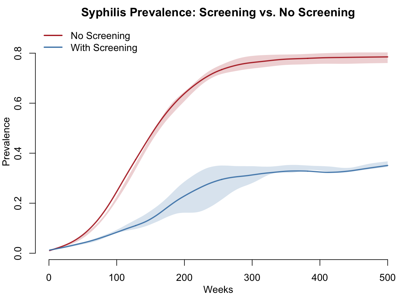
Stage Composition
The two-panel plot below shows the actively transmitting stages (left, primary + secondary + early latent, matching CDC’s surveillance definition of “infectious syphilis”) and the non-transmitting reservoir (right, incubating + late latent). With screening, both compartments are substantially reduced; without screening, the late latent compartment grows unchecked as asymptomatic cases accumulate.
par(mfrow = c(1, 2), mar = c(3, 3, 2, 1), mgp = c(2, 1, 0))

plot(sim_noscr, y = "infectious.num",
     main = "Infectious Stages (primary + secondary + early latent)",
     ylab = "Count", xlab = "Weeks",
     mean.col = "firebrick", mean.lwd = 2, mean.smooth = TRUE,
     qnts.col = "firebrick", qnts.alpha = 0.2, qnts.smooth = TRUE,
     legend = FALSE)
plot(sim_scr, y = "infectious.num", add = TRUE,
     mean.col = "steelblue", mean.lwd = 2, mean.smooth = TRUE,
     qnts.col = "steelblue", qnts.alpha = 0.2, qnts.smooth = TRUE,
     legend = FALSE)
legend("topleft", legend = c("No Screening", "With Screening"),
       col = c("firebrick", "steelblue"), lwd = 2, cex = 0.8, bty = "n")

plot(sim_noscr, y = "latent.num",
     main = "Non-transmitting (incubating + late latent)",
     ylab = "Count", xlab = "Weeks",
     mean.col = "firebrick", mean.lwd = 2, mean.smooth = TRUE,
     qnts.col = "firebrick", qnts.alpha = 0.2, qnts.smooth = TRUE,
     legend = FALSE)
plot(sim_scr, y = "latent.num", add = TRUE,
     mean.col = "steelblue", mean.lwd = 2, mean.smooth = TRUE,
     qnts.col = "steelblue", qnts.alpha = 0.2, qnts.smooth = TRUE,
     legend = FALSE)
legend("topleft", legend = c("No Screening", "With Screening"),
       col = c("firebrick", "steelblue"), lwd = 2, cex = 0.8, bty = "n")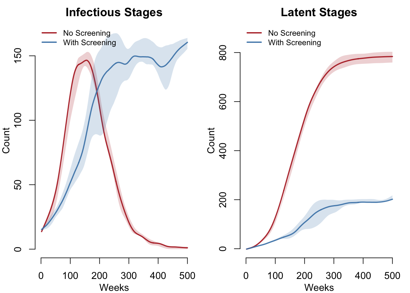
Summary Table
The table below compares key epidemiological outcomes between the two scenarios at the end of the simulation.
df_scr <- as.data.frame(sim_scr)
df_noscr <- as.data.frame(sim_noscr)
last_t <- max(df_scr$time)

data.frame(
  Metric = c("Mean prevalence",
             "Peak prevalence",
             "Cumulative new infections",
             "Total recoveries",
             "Peak latent reservoir"),
  Screening = c(round(mean(df_scr$prev, na.rm = TRUE), 3),
                round(max(df_scr$prev, na.rm = TRUE), 3),
                sum(df_scr$si.flow, na.rm = TRUE),
                sum(df_scr$rec.flow, na.rm = TRUE),
                max(df_scr$latent.num, na.rm = TRUE)),
  No_Screening = c(round(mean(df_noscr$prev, na.rm = TRUE), 3),
                   round(max(df_noscr$prev, na.rm = TRUE), 3),
                   sum(df_noscr$si.flow, na.rm = TRUE),
                   sum(df_noscr$rec.flow, na.rm = TRUE),
                   max(df_noscr$latent.num, na.rm = TRUE))
)
Metric Screening No_Screening
1 Mean prevalence 0.087 0.489
2 Peak prevalence 0.229 0.749
3 Cumulative new infections 6388.000 4892.000
4 Total recoveries 5550.000 1284.000
5 Peak latent reservoir 122.000 748.000
Note
Cumulative infections may be higher with screening because recovered individuals return to the susceptible pool and can be reinfected. This is a feature of SIS-type dynamics. The relevant public health metric is prevalence (the disease burden at any point in time), not cumulative incidence.
Parameters
Transmission Parameters
| Parameter | Description | Value |
|---|---|---|
inf.prob.incubating |
Per-act transmission probability during incubation (pre-chancre); zero by default per CDC mucocutaneous-lesion framing | 0 |
inf.prob.early |
Per-act transmission probability for primary and secondary stages (mucocutaneous lesions present) | 0.18 |
inf.prob.latent |
Per-act transmission probability for early latent stage (residual transmission via clinical relapses) | 0.09 |
act.rate |
Number of acts per partnership per timestep | 2 |
Stage Progression Parameters
| Parameter | Description | Value |
|---|---|---|
ipr.rate |
Incubating to primary transition rate | 1/4 (~4 week duration) |
prse.rate |
Primary to secondary transition rate | 1/9 (~9 week duration) |
seel.rate |
Secondary to early latent transition rate | 1/17 (~17 week duration) |
elll.rate |
Early latent to late latent transition rate | 1/22 (~22 week duration) |
llter.rate |
Late latent to tertiary transition rate | 1/1508 (~29 year duration) |
Symptom and Treatment Parameters
| Parameter | Description | Value |
|---|---|---|
pri.sym |
Probability of developing symptoms per week in primary stage | 0.205 |
sec.sym |
Probability of developing symptoms per week in secondary stage | 0.106 |
early.trt |
Weekly probability of treatment given symptoms (primary/secondary) | 0.8 |
late.trt |
Weekly probability of treatment given symptoms (tertiary) | 1.0 |
scr.rate |
Weekly probability of screening (asymptomatic infected population) | 1/52 (~yearly) |
Module Execution Order
At each timestep, EpiModel executes the modules in the order specified by module.order in control.net():
| Order | Module | Function | Purpose |
|---|---|---|---|
| 1 | Network resimulation | resim_nets.FUN |
Resimulates the dynamic network for the current timestep (built-in) |
| 2 | Infection | infection.FUN |
Stage-dependent transmission across discordant partnerships |
| 3 | Progression | progress.FUN |
Advances infected individuals through syphilis stages |
| 4 | Treatment and screening | tnt.FUN |
Symptomatic treatment and population-level screening |
| 5 | Prevalence | prevalence.FUN |
Tabulates compartment sizes and saves summary statistics (built-in) |
Next Steps
This model provides a foundation for more detailed syphilis modeling. Possible extensions include:
- Vital dynamics: Adding births and deaths to allow the epidemic to reach endemic equilibrium over longer time horizons. See the SI with Vital Dynamics example.
- Heterogeneous progression: Varying progression rates by individual attributes such as age or immune status.
- Partial immunity: Modeling reinfection with reduced susceptibility after recovery.
- Partner notification: Adding contact tracing as an additional pathway to treatment, complementing both symptomatic diagnosis and population screening.
- Vaccination: Adding a vaccination compartment for syphilis prevention. See the SEIR with All-or-Nothing Vaccination example for vaccination modeling patterns.