flowchart LR
    S["<b>S</b>"] -->|"infection<br/>(household or community)"| E
    E["<b>E</b>"] -->|"~4 days, 70%"| Ip
    E -->|"~4 days, 30%"| Ia["<b>I_a</b><br/>asymp"]
    Ip["<b>I_p</b><br/>presymp"] -->|"~2 days"| Is["<b>I_s</b><br/>symp"]
    Is -->|"~7 days"| R["<b>R</b>"]
    Ia -->|"~7 days"| R

    style S fill:#3498db,color:#fff
    style E fill:#9b59b6,color:#fff
    style Ip fill:#f39c12,color:#fff
    style Is fill:#e74c3c,color:#fff
    style Ia fill:#e67e22,color:#fff
    style R fill:#27ae60,color:#fff
Age-Stratified RSV on a Household + Community Network
RSV
SEIR
multilayer
households
age structure
vaccination
advanced
A respiratory virus example: a population built from households (each a fixed clique) plus a TERGM community layer with a fully specified age-mixing matrix, age-based prior immunity, recorded transmission chains, and age-targeted products (older-adult vaccine, infant antibody) with separate infection-blocking and severity-reducing effects, compared with household cocooning, an equal-dose random comparator, and an NPI.
Overview
Respiratory syncytial virus (RSV) is a respiratory virus that spreads through everyday close contact rather than through the long-duration partnerships that most Gallery examples model. Nearly everyone is infected by age 2 and reinfected throughout life, so susceptibility and severity are strongly age-dependent: severe disease concentrates in infants and older adults, while children carry most transmission. Since 2023 there has been a portfolio of age-targeted products (long-acting monoclonal antibodies for infants, maternal vaccination, and vaccines for older adults), and public health agencies use scenario models to ask which products avert the most hospitalizations.
This example builds a single-season RSV model with three features that no other Gallery example combines:
A household plus community network. The population is generated household by household, and every household is a fixed clique: a static contact layer that is not an ERGM and is never resimulated. On top of it runs a community layer, a TERGM of transient daily contacts in which every cell of the age-by-age mixing matrix is set through
nodemix. The example shows how to combine a hand-built static layer with a simulated dynamic one insidenetsim, and how to record every transmission with its layer so that who-infects-whom can be analyzed afterwards.A five-stratum age structure that governs contact, susceptibility, severity, and eligibility. Infants (< 1 year), young children (1-4), school-age children (5-17), adults (18-64), and older adults (65+). Age is used as a proxy for prior exposure history, so older groups are less susceptible per contact.
Age-targeted and household-targeted interventions. The older-adult vaccine and the infant monoclonal antibody each reduce the per-contact probability of infection (which also protects others) and the risk of hospitalization given infection (which protects only the recipient). Because households are explicit, a cocooning scenario that immunizes the co-residents of infants is definable, and an equal-dose comparator that immunizes people of the same ages chosen at random shows what the household link itself contributes. A community-layer non-pharmaceutical intervention (NPI) is included as a comparison.
The policy question is the one asked of RSV scenario models: in one season, which strategy averts the most hospitalizations, how many doses does each hospitalization averted cost, and how much of each product’s effect is indirect? The example also shows how to answer it honestly on a stochastic network model, with Monte Carlo intervals on every intervention effect.
NoteHow this relates to other RSV scenario tools
The RSV Scenario Modeling Hub and the R.Scenario.Vax package use age-structured compartmental models that are calibrated to RSV-NET hospitalizations and include births, maternal immunity, exposure-history immunity, seasonal forcing, and waning of product protection across seasons. Those tools are built to project hospitalizations for a specific place and season. This example trades those features for an explicit contact network, so that transmission within households can be separated from transmission in the community and interventions can be targeted at the individual or household level. It follows the Hub’s convention of stating product effectiveness against hospitalization, but its parameters are illustrative and it is not calibrated to surveillance data. Treat it as a template for building an RSV network model, not as a forecasting tool.
TipDownload and run the standalone scripts
- model.R: main simulation script
- module-fx.R: custom module functions
model.R sources module-fx.R from examples/rsv/ when run from the repository root and from the working directory otherwise, so the two downloaded files can sit in one folder. Sourcing the script interactively (for example in RStudio) uses the full settings on this page (N = 10000, ten simulations, 150 days, two to three minutes on a laptop). Rscript is not interactive and uses the small continuous-integration settings (N = 1000, one simulation, 50 days, well under a minute) whose results are not meant to be interpreted; to get the full settings from the command line, pass R code that defines run_full as the first argument:
Rscript model.R "run_full <- TRUE"Model Structure
Disease Compartments
| Status | Sub-stage | Description |
|---|---|---|
| S | Susceptible (per-contact susceptibility scaled by age) | |
| E | Exposed, latent (mean 4 days) | |
| I | inf_stage = "ip" |
Presymptomatic infectious (mean 2 days), for infections that will become symptomatic |
| I | inf_stage = "is" |
Symptomatic infectious (mean 7 days) |
| I | inf_stage = "ia" |
Asymptomatic infectious (mean 7 days, half as infectious); these infections skip the presymptomatic stage |
| R | Recovered, immune for the rest of the season |
The standard status attribute holds the SEIR compartment and an additional inf_stage attribute carries the I substage. Whether an infection will be symptomatic is decided when it leaves E: 70% enter the presymptomatic stage and then become symptomatic, and 30% are asymptomatic throughout. Every stage duration is geometric with the stated mean, because each transition is a daily Bernoulli draw. The presymptomatic and asymptomatic stages are what make NPIs relevant for respiratory pathogens: isolation triggered by symptoms misses both.
Age Structure
Each age group differs in four ways: its household and community contact rates, its per-contact susceptibility (a proxy for prior immunity), its hospitalization risk per infection, and its eligibility for a product. The contact degrees below are realized values at N = 10,000: the household degree follows from the household mix, and the community degree from the fitted ERGM (see the diagnostics sections).
| Group | Ages | Share of N | Household degree | Community degree | Susceptibility (sus.mult) |
Hospitalization risk per infection | Product |
|---|---|---|---|---|---|---|---|
| infant | < 1 | 1.2% | 2.8 | 2.3 | 1.00 | 0.030 | monoclonal antibody |
| young | 1-4 | 5.2% | 2.6 | 5.3 | 0.55 | 0.006 | |
| school | 5-17 | 18% | 2.7 | 6.9 | 0.16 | 0.001 | |
| adult | 18-64 | 58% | 1.8 | 5.0 | 0.07 | 0.004 | |
| elderly | 65+ | 18% | 0.9 | 3.1 | 0.13 | 0.045 | vaccine |
Anyone other than an infant who lives with an infant is eligible for the hypothetical cocooning product.
Hospitalization is not a compartment. Expected hospitalizations are computed after the simulation as infections times the per-infection risk, with the risk further reduced for immunized people. This keeps the disease model simple while letting the analysis report the burden-weighted outcome that RSV policy is judged on.
Setup
suppressMessages(library(EpiModel))

# These are the full settings of the standalone model.R. The population is
# larger than in other Gallery examples because the outcome strata at the
# age extremes are small: infants are about 1% of N.
N <- 10000
nsims <- 10
ncores <- 5
nsteps <- 150
# The custom modules (init_attrs, infect, progress) used in control.net().
# The excerpts shown under "Custom Modules" are pulled from this file.
source("module-fx.R")Population and Households
The population is built from households rather than from individuals. Each entry in hh_types is a household type: the name lists its members by age group and the value is the probability that a sampled household is of that type. This is the simplest way to get a joint distribution of ages within households, which is what the household layer needs: every infant lives with at least one adult, about 60% of infants have an older sibling (in the United States about 60% of births are second or later births), about 10% of infants live with a single adult, some infants have a co-resident grandparent, and about 28% of older adults live alone. The mix was chosen so that the person-level age shares approximate the United States, with a mean household size of 2.3.
hh_types <- c(
  "adult"                          = 0.150,
  "adult adult"                    = 0.182,
  "adult adult adult"              = 0.050,
  "elderly"                        = 0.120,
  "elderly elderly"                = 0.120,
  "adult elderly"                  = 0.030,
  "adult adult infant"             = 0.007,
  "adult adult infant young"       = 0.007,
  "adult adult infant school"      = 0.006,
  "adult adult infant young school" = 0.003,
  "adult adult infant elderly"     = 0.002,
  "adult infant"                   = 0.002,
  "adult infant young"             = 0.001,
  "adult adult young"              = 0.030,
  "adult adult young young"        = 0.010,
  "adult adult young school"       = 0.035,
  "adult young"                    = 0.010,
  "adult adult school"             = 0.060,
  "adult adult school school"      = 0.070,
  "adult adult school school school" = 0.020,
  "adult school"                   = 0.035,
  "adult school school"            = 0.020,
  "adult adult school elderly"     = 0.020,
  "adult adult young elderly"      = 0.010
)
stopifnot(abs(sum(hh_types) - 1) < 1e-8)
From household types to a static clique layer
Two helpers do the work. The first samples households until the population reaches N and returns each person’s age group and household id, with households on consecutive node ids. The second turns the household ids into an edgelist by connecting every pair of co-residents, so each household is a clique. That edgelist is the household layer: there is no ERGM to fit and nothing to resimulate.
generate_households <- function(N, hh_types, seed = NULL) {
  if (!is.null(seed)) set.seed(seed)
  members <- strsplit(names(hh_types), " ")
  sizes <- lengths(members)
  n_draw <- ceiling(1.5 * N / sum(hh_types * sizes)) + 10
  draw <- sample.int(length(hh_types), n_draw, replace = TRUE, prob = hh_types)
1  draw <- draw[seq_len(which(cumsum(sizes[draw]) >= N)[1])]
  age <- unlist(members[draw])[1:N]
  hh_id <- rep(seq_along(draw), sizes[draw])[1:N]
  list(age = age, hh_id = hh_id)
}

household_edgelist <- function(hh_id) {
  members <- split(seq_along(hh_id), hh_id)
2  members <- members[lengths(members) > 1]
  el <- do.call(rbind, lapply(members, function(m) t(combn(m, 2))))
  unname(el)
}

pop <- generate_households(N, hh_types, seed = 123)
age <- pop$age
hh_id <- pop$hh_id
hh_el <- household_edgelist(hh_id)

counts <- table(factor(age, levels = c("adult", "elderly", "infant",
                                       "school", "young")))
counts- 1
-
Households are sampled until their cumulative size reaches
N; at most the last household is cut short by the truncation toN. - 2
- Single-person households contribute no edges. They still exist as nodes with a household id, and their only contacts are in the community layer.
  adult elderly  infant  school   young
   5799    1812     117    1756     516
Household-layer diagnostics
Because the layer is a fixed edgelist, its diagnostics are direct: the household size distribution and the mean degree by age are read from the data rather than from simulated networks.
table(tabulate(hh_id))
   1    2    3    4    5
1157 1660  728  706  103
hh_deg <- tabulate(c(hh_el[, 1], hh_el[, 2]), nbins = N)
deg_hh_by_age <- round(tapply(hh_deg, age, mean), 2)
deg_hh_by_age adult elderly infant school young
1.76 0.85 2.76 2.74 2.61
NoteWhy a clique layer rather than a long-duration ERGM
An earlier version of this example modeled family contacts as a second TERGM layer with a long mean tie duration. That gives the right degree by age but not the right structure: the ties form a sparse random graph over the whole population, so an infected adult’s family ties reach into many different families, and an infant’s two “parents” are unlikely to be each other’s partners. Real household transmission is closed: the people an infant can infect at home are exactly the people who can infect it. A clique layer has that closure by construction, which is why household secondary attack rates, sibling-to-infant introduction, and household-targeted strategies (cocooning) can only be represented this way. The cost is that the layer has no dynamics and no ERGM; in a model with births or migration, arrivals have to be wired into an existing household by hand.
The Community Layer with nodemix
The community layer is a TERGM of transient daily contacts. Its formation model is ~edges + nodemix("age"), which gives every cell of the age-by-age mixing matrix its own target statistic. Both age and hh_id are set as vertex attributes so that netsim carries them into the simulation, where the modules read them with get_attr().
Why every cell is targeted
nodemix lets you target any subset of the mixing cells. It is tempting to constrain only the cells that carry epidemiological signal and leave the others free. The catch is what “free” means: the untargeted cells share the baseline edges coefficient, so whatever edge count remains after the targeted cells are filled is spread across the untargeted dyads at a uniform per-dyad rate. Because the adult-by-elderly block contains far more dyads than any other cross-age block, a sparse specification quietly gives older adults among the highest degrees in the layer, and infants a community degree several times what was intended. Targeting the full matrix fixes the degree of every age group by design, and the diagnostics below verify it.
The cell ordering ergm uses for nodemix is the upper triangle of the mixing matrix, column-major, with alphabetical levels. Rather than hard-coding the 15 cell names, we read them from ergm:
nw <- network_initialize(N)
nw <- set_vertex_attribute(nw, "age", age)
nw <- set_vertex_attribute(nw, "hh_id", hh_id)

cells <- sub("^mix\\.age\\.", "",
             names(summary(nw ~ nodemix("age", levels2 = TRUE))))
cells
[1] "adult.adult" "adult.elderly" "elderly.elderly" "adult.infant"
[5] "elderly.infant" "infant.infant" "adult.school" "elderly.school"
[9] "infant.school" "school.school" "adult.young" "elderly.young"
[13] "infant.young" "school.young" "young.young" From a contact profile to cell targets
Contact rates are easier to think about per person than per cell, so the layer is specified as a profile: each entry a.b is the mean number of b-partners per a-node. The helper multiplies by the size of group a (halving within-group cells, where each edge is counted from both ends), maps the pair to its canonical cell name, and rounds to whole edges so that ergm can match the targets exactly. Cross-age entries are written from the perspective of the smaller group because that is the number with an intuitive meaning (each school-age child has 1.5 adult community contacts; each adult has 0.5 school-age contacts).
mix_targets <- function(profile, counts, cells) {
  out <- setNames(numeric(length(cells)), cells)
  for (nm in names(profile)) {
    ab <- strsplit(nm, ".", fixed = TRUE)[[1]]
    n_a <- as.numeric(counts[ab[1]])
    e <- if (ab[1] == ab[2]) n_a * profile[[nm]] / 2 else n_a * profile[[nm]]
    cell <- paste(sort(ab), collapse = ".")
    stopifnot(cell %in% cells)
    out[cell] <- out[cell] + e
  }
  pmax(round(out), 1)
}
Daily contacts outside the household, with the strong age assortativity seen in contact surveys (Mossong et al. 2008). School-age children have the highest degree and mix mostly with each other; this is the model’s school amplifier. Infants have the fewest community contacts: non-household caregivers and, for the share of infants in child care, other infants and young children.
com_profile <- c(
1  school.school   = 5.0,   # classmates
  adult.adult     = 4.0,   # workplace, social
  young.young     = 2.5,   # child care
  elderly.elderly = 1.5,
  school.adult    = 1.5,   # teachers, coaches, friends' parents
  young.adult     = 2.0,   # child care staff
  elderly.adult   = 1.2,
  school.elderly  = 0.3,   # grandparents
  young.school    = 0.5,
  infant.adult    = 1.0,   # non-household caregivers
2  infant.young    = 0.6,   # child care
  infant.infant   = 0.3,   # child care
  infant.school   = 0.2,
  infant.elderly  = 0.2,
  young.elderly   = 0.3
)
com_targets <- mix_targets(com_profile, counts, cells)- 1
- The magnitude of within-school contact is a model choice, not a calibrated estimate. Changing it is the quickest way to see how much the school amplifier drives infections in the other age groups.
- 2
- The infant entries were raised, relative to an earlier version, until the baseline infant attack rate landed in the published range (see the parameter table below). Whether an infant’s exposure comes mostly from home or from child care is a setting-specific question, and the transmission matrix reported in the analysis shows what these values imply.
WarningTwo simplifications in the community layer
Contacts do not persist. Every community tie lasts one day, so classmates and coworkers are redrawn daily. The layer reproduces the daily contact rate by age but not the persistence of real school and workplace contacts. This is the simplest TERGM specification and a consequential one: a longer tie duration at the same mean degree would make repeated contacts with the same infectious person more likely and spread infection through fewer households. Varying duration in dissolution_coefs() while holding the profile fixed is a worthwhile experiment (see Next Steps).
Co-residents can also meet in the community. The ERGM does not exclude household pairs from the community layer. The expected number of community edges that fall on a household pair is the number of household pairs times the per-dyad tie probability, which is a few edges per day among the roughly 25,000 in the layer, and those pairs already transmit at the higher household rate. Excluding them would need an ergm constraint on the household dyads and was not worth the complexity here.
Fitting the community layer
levels2 = -1 drops the first cell (adult.adult) as the reference; its count is implied by the edges target minus the other 14 cells. Community ties last one day.
formation <- ~edges + nodemix("age", levels2 = -1)

1san_ctrl <- control.ergm(SAN = control.san(SAN.maxit = 20,
                                           SAN.nsteps = 2^21))

coef.diss_com <- dissolution_coefs(~offset(edges), duration = 1)

est_com <- netest(nw, formation,
                  target.stats = c(sum(com_targets),
                                   as.numeric(com_targets[-1])),
                  coef.diss = coef.diss_com,
set.control.ergm = san_ctrl, verbose = FALSE)- 1
- SAN budget. With 14 targeted cells, ergm’s default simulated annealing step sometimes cannot hit every target exactly, and ergm then falls back to MCMC estimation, which takes minutes for a model that is dyad-independent and could be fit by maximum pseudolikelihood in seconds. Giving SAN more iterations and steps lets it match the targets, after which the fast fit is used.
Community-layer diagnostics
The check that the profile translated into the intended age-specific contact rates. nodefactor("age", levels = TRUE) returns the total degree of each group, which divided by group size is the mean degree. The household row is repeated for comparison.
mean_degree_by_age <- function(est, counts) {
  dx <- netdx(est, nsims = 10, dynamic = FALSE, verbose = FALSE,
              nwstats.formula = ~edges + nodemix("age", levels2 = TRUE) +
                                 nodefactor("age", levels = TRUE))
  st <- colMeans(do.call(rbind, lapply(dx$stats, as.matrix)))
  st <- st[grep("^nodefactor", names(st))]
  names(st) <- sub("nodefactor.age.", "", names(st))
  round(st / as.numeric(counts[names(st)]), 2)
}
deg_by_age <- rbind(household = deg_hh_by_age[names(counts)],
                    community = mean_degree_by_age(est_com, counts))
knitr::kable(deg_by_age, caption = "Realized mean degree by age group and layer")| adult | elderly | infant | school | young | |
|---|---|---|---|---|---|
| household | 1.76 | 0.85 | 2.76 | 2.74 | 2.61 |
| community | 4.99 | 3.08 | 2.25 | 6.89 | 5.34 |
Custom Modules
Three custom modules: init_attrs (one-shot setup of immunization status and the I substage), infect (S to E across both layers, with every transmission recorded), and progress (E to Ip to Is to R or E to Ia to R, plus the age-stratified counters). Full code is in module-fx.R; the parts that carry the model’s logic are below.
infect: a static layer and a simulated layer, walked the same way
The household edgelist is passed to netsim as the parameter hh.pairs, so the infection module can read it with get_param() on every step, exactly as it reads the community layer’s current edgelist with get_edgelist(). Everything downstream of that line is layer-agnostic. Each layer contributes its successful exposures to one table, and the infections are resolved after both layers have been walked.
hh_el <- get_param(dat, "hh.pairs")
del <- NULL
for (k in 1:2) {
1  el <- if (k == 1) hh_el else get_edgelist(dat, network = 1)
  if (is.null(el) || nrow(el) == 0) next

  head <- el[, 1]; tail <- el[, 2]
2  if (k == 2 && com.contact.mult < 1) {
    keep <- which(rbinom(nrow(el), 1, com.contact.mult) == 1)
    head <- head[keep]; tail <- tail[keep]
  }

  # ... identify (sus, inf) pairs on this layer's discordant edges ...

  base.p <- layer_probs[k]
  stages <- inf_stage[inf]
3  trans.p <- ifelse(stages %in% "ia", base.p * asymp.mult, base.p)

4  trans.p <- trans.p * as.numeric(sus.mult[age[sus]])
  vax <- vax_status[sus]
  eff <- rep(0, length(sus))
  eff[!is.na(vax) & vax == "elderly_vax"] <- eff.inf.elderly
  eff[!is.na(vax) & vax == "infant_proph"] <- eff.inf.infant
  eff[!is.na(vax) & vax == "cocoon"] <- eff.inf.cocoon
5  trans.p <- trans.p * (1 - eff)

  hit <- which(rbinom(length(trans.p), 1, trans.p) == 1)
  if (length(hit) > 0) {
    del <- rbind(del, data.frame(sus = sus[hit], inf = inf[hit], layer = k))
  }
}

if (!is.null(del) && nrow(del) > 0) {
6  del <- del[sample.int(nrow(del)), , drop = FALSE]
  del <- del[!duplicated(del$sus), , drop = FALSE]

  new_inf <- del$sus
  status[new_inf] <- "e"
  infTime[new_inf] <- at
  dat <- set_attr(dat, "status", status)
  dat <- set_attr(dat, "infTime", infTime)

7  del$at <- at
  del$susAge <- age[del$sus]
  del$infAge <- age[del$inf]
  del$infTime <- infTime[del$inf]
  dat <- set_transmat(dat, del, at)
  # ... per-layer counts for the epi output ...
}- 1
-
Two sources, one loop. Layer 1 is the fixed household edgelist from the parameter list; layer 2 is the community TERGM, the only network
netsimknows about, hencenetwork = 1. Walking each layer separately, instead of callingdiscord_edgelist(), is what allows different transmission probabilities per layer. - 2
-
NPI contact thinning. While the NPI is active, each community edge is kept with probability
npi.contact.mult, an approximation to a reduced contact rate.layer_probs[2]is also multiplied by(1 - npi.mask.efficacy)during the window. - 3
- Infectious-side modifier. Asymptomatic partners transmit at half the rate.
- 4
-
Age-specific susceptibility. The proxy for prior immunity: the per-contact probability is scaled by
sus.multfor the susceptible partner’s age, relative to a never-infected infant. - 5
- Infection-blocking component of immunization. A leaky reduction for immunized susceptibles. This is the only product effect that reduces transmission to others, and for cocooning it is the whole effect.
- 6
- Competing exposures. Every discordant edge on both layers is a separate Bernoulli trial. A susceptible node with more than one successful exposure in the same step is infected once, and its infector, and hence its layer, is a uniform random draw among the successes: shuffle the successful exposures, then keep the first row per node. This is the tie-breaking rule EpiModel’s built-in infection module uses. An earlier version attributed every simultaneous success to the household, which biased the layer shares.
- 7
-
Transmission record.
set_transmat()stores the rows for this step, andnetsimbinds them into one table per simulation thatget_transmat()returns. Extra columns ride along, so the record carries the layer, both ages, and the infector’s own infection time (1 for the seeds), which is what the who-infects-whom analysis below uses.
init_attrs: household ids make household targeting definable
Every co-resident of an infant, of any age, is eligible for the cocooning product. The comparator draws the same number of people of the same ages from the whole population, so the two arms differ only in whether the recipients live with an infant.
infant_hh <- unique(hh_id[active == 1 & age == "infant"])
elig_c <- which(active == 1 & age != "infant" & hh_id %in% infant_hh)
if (length(elig_c) > 0 && cocoon.cov > 0) {
  hit <- elig_c[rbinom(length(elig_c), 1, cocoon.cov) == 1]
  if (cocoon.random == 1 && length(hit) > 0) {
    n_by_age <- table(age[hit])
    hit <- unlist(lapply(names(n_by_age), function(a) {
      pool <- which(active == 1 & age == a)
      pool[sample.int(length(pool), n_by_age[[a]])]
    }))
  }
  vax_status[hit] <- "cocoon"
}progress: counters that make the analysis possible
Hospitalizations are computed after the fact, so progress records cumulative incident infections by age, and separately among immunized infants and older adults, so that the severity-reducing component of each product can be applied only where it belongs and the realized effectiveness among recipients can be computed. Seed infections from init.net() carry infTime = 1 and are excluded. The numbers of immunized people are recorded too, so that doses are counted from the simulation rather than as coverage times a population.
incident <- is_active & !is.na(infTime) & infTime > 1
for (a in c("infant", "young", "school", "adult", "elderly")) {
  dat <- set_epi(dat, paste0("cuminf.", a), at, sum(incident & age == a))
}
inf_prot <- is_active & vax_status %in% "infant_proph"
eld_prot <- is_active & vax_status %in% "elderly_vax"
dat <- set_epi(dat, "cuminf.infant.prot", at, sum(incident & inf_prot))
dat <- set_epi(dat, "cuminf.elderly.prot", at, sum(incident & eld_prot))
dat <- set_epi(dat, "n.infant.prot", at, sum(inf_prot))
dat <- set_epi(dat, "n.elderly.prot", at, sum(eld_prot))
dat <- set_epi(dat, "n.cocoon", at, sum(is_active & vax_status %in% "cocoon"))
Module order
EpiModel’s default order runs user-supplied modules before the built-in ones, which here would run progress ahead of infect within each step. The order is set explicitly in control.net() so that each step runs
resim_nets -> summary_nets -> initAttr -> infection -> progress -> nwupdate -> prevalenceWith infection before progression, progress requires infTime < at for the E to I transition, which excludes infections written in the same step and guarantees at least one step in E.
Disease, Immunity, and Intervention Parameters
Natural history. Mean latent period 4 days (the pooled median incubation period for RSV is 4.4 days; Lessler et al. 2009), presymptomatic 2 days, symptomatic or asymptomatic 7 days (mean shedding of 6.7 days in hospitalized infants; Hall et al. 1976), 30% of infections asymptomatic at half infectiousness. Every duration is geometric. The natural history does not vary by age, although infants shed longer and adults shorter; age-dependent durations are a natural extension.
Seasonal forcing. RSV is strongly seasonal, and its seasons end because transmissibility falls, not only because susceptible people run out. Both layers’ transmission probabilities are multiplied by a cosine with a period of one year, \(1 + \text{seas.amp} \cos(2\pi (t - \text{seas.peak}) / 365)\), with the peak on day 1 so that the run starts at the top of the season and follows its decline. The forcing does two things for the example. It gives the epidemic a season-shaped curve that is over by about day 120, so the outcomes reported through day 150 are final sizes rather than snapshots of an ongoing epidemic. And it narrows the final-size distribution: without forcing, the same attack rates require an epidemic that barely grows, and the between-simulation coefficient of variation of season totals roughly doubles, which makes every intervention comparison noisier. The Scenario Modeling Hub asks teams to include their own seasonality; the amplitude here is illustrative.
Prior immunity. In the Houston Family Study 69% of infants were infected in their first year and 83% in their second, and by age 4 the annual reinfection risk had fallen to about a third (Glezen et al. 1986); about 7% of healthy working adults (Hall et al. 2001) and 3-7% of healthy older adults (Falsey et al. 2005) are infected each year. Transmission models of RSV represent this with progressively reduced susceptibility after each infection (Pitzer et al. 2015). This example uses age as a proxy for exposure history: sus.mult scales per-contact susceptibility for each age group relative to a never-infected infant. The per-contact transmission probabilities, the forcing amplitude, and sus.mult were chosen together, by iterating the baseline scenario, so that the season-long attack rates land near that gradient: 50-70% of infants, 40-60% of 1-4 year olds, 20-30% of school-age children, 7-10% of adults (parents of young children run higher than the healthy-worker figure), and 3-7% of older adults. The baseline attack rates are reported below so that the reader can check the run in hand against these ranges. They are illustrative, not fitted to data.
Products. Each product has two leaky components, following how the products are evaluated in trials and how other RSV scenario models represent them: eff.inf reduces the per-contact probability of infection, and eff.hosp reduces the hospitalization risk given infection. Against a single exposure the two combine to \(1 - (1 - \text{eff.inf})(1 - \text{eff.hosp}) = 0.80\) for both products, the first-season effectiveness against hospitalization assumed by the RSV Scenario Modeling Hub (Round 4, 2026-27 season: 80% for infant monoclonals and for older-adult vaccines in the year of vaccination). That equality holds per exposure, not per season. Because eff.inf is leaky and acts per contact, a recipient who is exposed repeatedly over the season is protected against infection by less than eff.inf, so the product’s realized effectiveness against hospitalization over the season is an output of the model. The analysis computes it from the attack rates among immunized and unimmunized members of each group and reports it next to the 80% input. The split between the two components is an assumption: setting eff.inf = 0 and eff.hosp = 0.80 gives a product with the same per-exposure effectiveness, no indirect effect, and a realized effectiveness of exactly 80% by construction. The Gallery’s all-or-nothing and leaky vaccination examples treat the distinction at length.
Cocooning and its comparator. Every co-resident of an infant (parents, siblings, grandparents) receives a hypothetical product with the older-adult vaccine’s infection-blocking component (cocoon.eff.inf = 0.5) and no severity component. No product is currently recommended for this purpose, and maternal vaccination protects the infant through antibody transfer rather than by blocking the parent’s transmission. The scenario is here because it is the question an explicit household layer makes answerable: how much infant protection can blocking household transmission deliver, at most, compared with a product given to the infant? Complete coverage makes it an upper bound. The equal-dose comparator gives the same number of doses of the same product to people of the same ages drawn at random from the whole population, so the difference between the two arms is the value of the household link itself.
ImportantSimplifications relative to current guidance and trial evidence
- Eligibility. The model immunizes a random fraction of all infants and of all adults 65+. Current CDC guidance is nirsevimab (or clesrovimab) for infants entering their first RSV season, or maternal vaccination during pregnancy, and a single vaccine dose for adults 75+ and adults 50-74 at increased risk of severe disease. The model has no births, so the in-season birth cohort and maternal vaccination are not represented, and infants are one stratum rather than an age in months.
- Efficacy endpoints. Trials report efficacy against medically attended RSV lower respiratory tract illness: 74.5% for nirsevimab in the MELODY trial (Hammitt et al. 2022) and 79.5% pooled, with 77.3% against hospitalization (Simões et al. 2023); 82.6% for the adjuvanted older-adult vaccine (Papi et al. 2023) and 66.7% to 85.7% depending on case definition for the bivalent vaccine (Walsh et al. 2023). None of these trials measured protection against infection itself.
- Waning. Product protection is constant within the season. Nirsevimab protects for at least 150 days and the older-adult vaccines for more than one season with declining effectiveness, so a single-season model does not need waning, but a multi-season extension would.
- Household ties are unweighted. Within a household every pair transmits at the same per-contact probability, so a parent-infant tie and a sibling-infant tie are identical. Weighting ties by relationship is a natural extension once households are explicit.
Parameter provenance
| Parameter | Value | Units and endpoint | Basis | Status |
|---|---|---|---|---|
hh_types |
table above | probability of each household composition | person-level age shares and mean household size of the United States; sibling and living-alone shares | illustrative |
com_profile |
table above | daily community contacts per person, by age pair | qualitative pattern of POLYMOD (Mossong 2008): assortative, highest among school-age children | illustrative |
inf.prob.household, inf.prob.community |
0.35, 0.08 | annual-mean per-contact, per-day probability of transmission to a never-infected infant, scaled by the seasonal multiplier | tuned, with sus.mult and the forcing amplitude, to the attack-rate gradient below |
illustrative |
seas.amp, seas.peak |
0.5, day 1 | amplitude of the annual cosine forcing on both layers; day of peak transmissibility | RSV seasons are forced; the run starts at the peak and follows the decline | illustrative |
sus.mult |
1.00 / 0.55 / 0.16 / 0.07 / 0.13 | relative per-contact susceptibility (infant / young / school / adult / elderly) | tuned to season attack rates of 50-70%, 40-60%, 20-30%, 7-10%, 3-7% (Glezen 1986, Hall 2001, Falsey 2005) | illustrative |
ei.rate |
1/4 | mean latent period, days | RSV incubation 4.4 days (Lessler 2009) | literature |
ip.rate, ir.rate |
1/2, 1/7 | mean presymptomatic and symptomatic or asymptomatic periods, days | shedding about a week (Hall 1976) | approximate |
asymp.prob, asymp.inf.mult |
0.3, 0.5 | share asymptomatic; relative infectiousness | assumption | illustrative |
elderly.vax.eff.inf, elderly.vax.eff.hosp |
0.5, 0.6 | per-contact reduction in infection; reduction in hospitalization given infection | combine to 80% per exposure, the Hub’s first-year value; trials 67-83% against medically attended illness | Hub-aligned total, assumed split |
infant.proph.eff.inf, infant.proph.eff.hosp |
0.3, 0.71 | as above | combine to 80% per exposure, the Hub’s value; trials 74-80% | Hub-aligned total, assumed split |
cocoon.eff.inf |
0.5 | per-contact reduction in infection for co-residents of infants | hypothetical product | hypothetical |
| coverage | 50% of 65+, 60% of infants, 100% of infant co-residents | share immunized before the season | Hub “usual” coverage for 2026-27: 56% of infants, 50% of adults 75+; complete coverage for the hypothetical cocoon | Hub-aligned, simplified eligibility |
npi.mask.efficacy, npi.contact.mult |
0.4, 0.7 | community per-contact reduction; share of community contacts kept, days 30-90 | hypothetical | hypothetical |
hosp_rate |
0.030 / 0.006 / 0.001 / 0.004 / 0.045 | hospitalizations per infection, by age | chosen so the baseline lands near the RSV-NET age pattern | illustrative |
N, nsteps, seeds |
10,000; 150 days; 1% infectious at day 1 | population; season length; initial conditions | a five-month season; 1% seeds start the epidemic without a long stochastic lag | design |
1init <- init.net(i.num = round(0.01 * N))

param_base <- param.net(
2  inf.prob.household = 0.35,
  inf.prob.community = 0.08,
3  seas.amp = 0.5,
  seas.peak = 1,
  sus.mult = c(infant = 1.00, young = 0.55, school = 0.16,
               adult = 0.07, elderly = 0.13),
  asymp.inf.mult = 0.5,
  ei.rate = 1 / 4,
  ip.rate = 1 / 2,
  ir.rate = 1 / 7,
  asymp.prob = 0.3,
4  elderly.vax.coverage = 0,
  elderly.vax.eff.inf = 0.5,
  elderly.vax.eff.hosp = 0.6,
  infant.proph.coverage = 0,
  infant.proph.eff.inf = 0.3,
  infant.proph.eff.hosp = 0.71,
  cocoon.coverage = 0,
  cocoon.eff.inf = 0.5,
  cocoon.random = 0,
  npi.start = -1,
  npi.end = -1,
  npi.mask.efficacy = 0.4,
  npi.contact.mult = 0.7,
5  hh.pairs = hh_el
)

control <- control.net(
  type = NULL,
  nsims = nsims, ncores = ncores, nsteps = nsteps,
  tergmLite = TRUE,
  resimulate.network = TRUE,
  initAttr.FUN = init_attrs,
  infection.FUN = infect,
  progress.FUN = progress,
  module.order = c("resim_nets.FUN", "summary_nets.FUN", "initAttr.FUN",
                   "infection.FUN", "progress.FUN", "nwupdate.FUN",
                   "prevalence.FUN"),
  verbose = FALSE
)- 1
- One percent of the population is seeded as infectious at the start of the season, placed at random across ages. Seeds are excluded from the incidence counters.
- 2
-
Annual-mean per-contact, per-day transmission probabilities, which the seasonal multiplier scales up to 1.5 times at the start of the run. Household contacts are higher-intensity than community contacts. With
sus.mult = 0.07for adults, an adult living with one infectious household member has about a 20% chance of infection over a 9-day infectious period at the annual mean and about 29% at the seasonal peak; for a never-infected infant the corresponding risks are 98% and above 99%, so the household layer is close to saturating for infants and what matters is whether a co-resident gets infected at all. - 3
- Seasonal forcing: both layers’ probabilities are multiplied by \(1 + 0.5 \cos(2\pi (t - 1) / 365)\), so transmissibility starts at 1.5 times the annual mean on day 1 and falls to about 0.6 times it by day 150.
- 4
- Intervention coverages default to zero and the NPI window to inactive, so the base parameter set is the no-intervention scenario. Scenarios override these below.
- 5
-
The household edgelist rides along in the parameter list.
param.net()accepts non-scalar entries, anduse_scenario()leaves entries the scenario does not name untouched.
Scenarios
Seven scenarios on the same network with identical disease parameters. Product coverage follows the “usual” assumptions of the RSV Scenario Modeling Hub for the 2026-27 season (56% of infants receiving a monoclonal antibody, 50% of adults 75+ vaccinated). The household cocoon covers every co-resident of an infant; the random arm gives the same number of doses to people of the same ages drawn from the whole population. The NPI is a strong hypothetical: for days 30 to 90, community contacts are cut by 30% and the remaining community contacts transmit at 60% of the usual rate.
scenarios.df <- data.frame(
  .scenario.id          = c("none", "elderly_vax", "infant_proph", "both",
                            "cocoon", "cocoon_random", "npi"),
  .at                   = 0,
  elderly.vax.coverage  = c(0, 0.5, 0, 0.5, 0, 0, 0),
  infant.proph.coverage = c(0, 0, 0.6, 0.6, 0, 0, 0),
  cocoon.coverage       = c(0, 0, 0, 0, 1, 1, 0),
  cocoon.random         = c(0, 0, 0, 0, 0, 1, 0),
  npi.start             = c(-1, -1, -1, -1, -1, -1, 30),
  npi.end               = c(-1, -1, -1, -1, -1, -1, 90)
)
scenarios.list <- create_scenario_list(scenarios.df)

labels <- c(none = "No intervention",
            elderly_vax = "Older-adult vaccine (50%)",
            infant_proph = "Infant antibody (60%)",
            both = "Both products",
            cocoon = "Household cocoon (all co-residents of infants)",
            cocoon_random = "Same doses, random people of the same ages",
            npi = "NPI (days 30-90)")

sims <- list()
for (scn in scenarios.list) {
  sims[[scn$id]] <- netsim(est_com, use_scenario(param_base, scn),
                           init, control)
}
Analysis
From infections to hospitalizations
Expected hospitalizations in each simulation are infections times the age-specific risk, minus the severity reduction for infections among immunized people. The per-infection risks are illustrative, chosen so that the baseline season lands near the age pattern of RSV-NET hospitalization rates (highest in infants, then older adults, lowest in school-age children) given the attack rates above. The summary keeps one row per simulation for every quantity, which is what the Monte Carlo intervals below are built from. Doses are the numbers of people actually immunized in the simulation, and the number needed to immunize (NNI) is doses per hospitalization averted.
hosp_rate <- c(infant = 0.030, young = 0.006, school = 0.001,
               adult = 0.004, elderly = 0.045)
eff_hosp <- c(infant = param_base$infant.proph.eff.hosp,
              elderly = param_base$elderly.vax.eff.hosp)

age_groups <- c("infant", "young", "school", "adult", "elderly")
age_pop <- as.numeric(counts[age_groups])
names(age_pop) <- age_groups

summarize_scenario <- function(sim) {
  df <- as.data.frame(sim)
  last <- df[df$time == max(df$time), ]           # one row per simulation
  hosp_sim <- sapply(age_groups, function(a) {
    last[[paste0("cuminf.", a)]] * hosp_rate[a]
  })
  hosp_sim <- matrix(hosp_sim, ncol = length(age_groups),
                     dimnames = list(NULL, age_groups))
  for (a in c("infant", "elderly")) {
    hosp_sim[, a] <- hosp_sim[, a] -
      last[[paste0("cuminf.", a, ".prot")]] * hosp_rate[a] * eff_hosp[a]
  }
  inf <- sapply(age_groups, function(a) mean(last[[paste0("cuminf.", a)]]))
  attack_prot <- attack_unprot <- matrix(NA_real_, nrow(last), 2,
                                         dimnames = list(NULL, c("infant", "elderly")))
  for (a in c("infant", "elderly")) {
    n_p <- last[[paste0("n.", a, ".prot")]]
    i_p <- last[[paste0("cuminf.", a, ".prot")]]
    attack_prot[, a] <- ifelse(n_p > 0, i_p / n_p, NA)
    attack_unprot[, a] <- (last[[paste0("cuminf.", a)]] - i_p) / (age_pop[a] - n_p)
  }
  doses <- mean(last$n.elderly.prot + last$n.infant.prot + last$n.cocoon)
  hh_share_infant <- sum(df$se.flow.infant.hh, na.rm = TRUE) /
    sum(df$se.flow.infant.hh + df$se.flow.infant.com, na.rm = TRUE)
  active_end <- mean(last$e.num + last$ip.num + last$is.num + last$ia.num)
  list(inf = inf, attack = inf / age_pop,
       hosp = colMeans(hosp_sim), hosp_sim = hosp_sim,
       hosp_per100k = 1e5 * colMeans(hosp_sim) / age_pop,
       attack_prot = attack_prot, attack_unprot = attack_unprot,
       doses = doses, hh_share_infant = hh_share_infant,
       active_end = active_end, cuminf_end = sum(inf))
}

res <- lapply(sims, summarize_scenario)
Attack rates and hospitalization burden
All outcomes are cumulative through day 150. The last table in this section checks how much of the season was still in progress at that point.
attack_tbl <- sapply(res, function(r) round(100 * r$attack, 1))
knitr::kable(attack_tbl,
caption = "Cumulative attack rate through the end of the run by age group (%), mean of simulations")| none | elderly_vax | infant_proph | both | cocoon | cocoon_random | npi | |
|---|---|---|---|---|---|---|---|
| infant | 56.8 | 53.8 | 53.2 | 51.1 | 47.0 | 52.7 | 28.0 |
| young | 61.5 | 59.5 | 60.7 | 59.9 | 56.5 | 55.6 | 30.8 |
| school | 28.3 | 27.3 | 26.3 | 25.2 | 24.6 | 24.7 | 12.4 |
| adult | 9.4 | 8.9 | 9.0 | 8.9 | 8.4 | 8.2 | 4.4 |
| elderly | 5.4 | 3.6 | 5.1 | 3.6 | 4.9 | 4.4 | 2.6 |
The baseline column is the check against the literature ranges stated above (50-70%, 40-60%, 20-30%, 7-10%, and 3-7%): 56.8% of infants, 61.5% of young children, 28.3% of school-age children, 9.4% of adults, and 5.4% of older adults infected in the season. Young children land at the top of their range because siblings and child care expose them heavily in this model, and adults who live with children run above the healthy-worker attack rate; both are what an explicit household layer produces.
hosp100k_tbl <- rbind(
  sapply(res, function(r) round(r$hosp_per100k)),
  total = sapply(res, function(r) round(1e5 * sum(r$hosp) / N))
)
knitr::kable(hosp100k_tbl,
caption = "Expected hospitalizations per 100,000 population, by age group (rows) and scenario; the total row is per 100,000 of all ages")| none | elderly_vax | infant_proph | both | cocoon | cocoon_random | npi | |
|---|---|---|---|---|---|---|---|
| infant | 1705 | 1615 | 945 | 916 | 1410 | 1582 | 841 |
| young | 369 | 357 | 364 | 359 | 339 | 334 | 185 |
| school | 28 | 27 | 26 | 25 | 25 | 25 | 12 |
| adult | 38 | 36 | 36 | 36 | 33 | 33 | 17 |
| elderly | 243 | 128 | 228 | 129 | 219 | 199 | 115 |
| total | 110 | 86 | 97 | 78 | 97 | 95 | 53 |
The hospitalization rates are within the range that RSV-NET reports for a season: on the order of 1,000 to 2,500 per 100,000 in infants, 100 to 300 per 100,000 in adults 65+, tens per 100,000 in adults 18-64, and about 100 per 100,000 overall. Older adults and infants together account for 58% of baseline hospitalizations even though they are a fifth of the population. Because the per-infection risks were chosen to reproduce that pattern, the hospitalization table is not an independent check of the transmission model; the attack-rate table and the transmission matrix below are.
knitr::kable(t(sapply(res, function(r) round(100 * r$active_end / r$cuminf_end, 1))),
caption = "Infections still in progress (E or I) at the last day, as a percent of the season's cumulative infections")| none | elderly_vax | infant_proph | both | cocoon | cocoon_random | npi |
|---|---|---|---|---|---|---|
| 0.3 | 0.3 | 0.4 | 0.3 | 0.3 | 0.4 | 0.2 |
The observation window matters for interpretation. With 0.3% of the baseline season’s infections still in progress on day 150, the scenario comparisons are about final size rather than timing, and a strategy that only delayed infections would show up here as a larger in-progress share, which the NPI does not.
cols_scn <- c(none = "gray40", elderly_vax = "seagreen",
              infant_proph = "purple", both = "darkblue",
              cocoon = "darkorange", cocoon_random = "goldenrod",
              npi = "firebrick")
lty_scn <- c(none = 1, elderly_vax = 1, infant_proph = 1, both = 1,
             cocoon = 1, cocoon_random = 2, npi = 1)
par(mfrow = c(2, 3), mar = c(3, 3.5, 2, 1), mgp = c(2.2, 0.7, 0))
for (a in age_groups) {
  col_name <- paste0("cuminf.", a)
  curves <- lapply(names(sims), function(s) {
    df <- as.data.frame(sims[[s]])
    tapply(df[[col_name]], df$time, mean, na.rm = TRUE) / age_pop[a]
  })
  names(curves) <- names(sims)
  max_y <- max(sapply(curves, max, na.rm = TRUE))
  plot(NA, xlim = c(1, nsteps), ylim = c(0, max(max_y, 0.01) * 1.05),
       xlab = "Day", ylab = "Cumulative attack rate",
       main = paste0(toupper(substr(a, 1, 1)), substr(a, 2, nchar(a)),
                    " (N=", age_pop[a], ")"))
  for (s in names(sims)) {
    lines(as.numeric(names(curves[[s]])), curves[[s]], lwd = 2,
          col = cols_scn[s], lty = lty_scn[s])
  }
}
plot.new()
legend("center", legend = labels, col = cols_scn, lwd = 2, lty = lty_scn,
       bty = "n", cex = 0.8)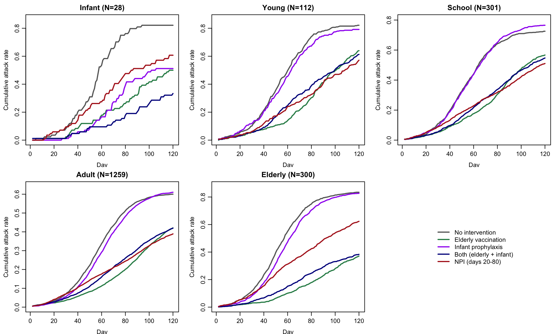
The product scenarios move mainly their own panel: the infant antibody lowers the infant curve and the older-adult vaccine lowers the elderly curve. The household cocoon lowers the infant curve without immunizing any infant, and the random arm, with the same doses, moves it much less. The NPI lowers every panel because it acts on the children who feed infections into the other groups. Movements in the untargeted panels are within the between-simulation noise quantified below.
cols_age <- c(infant = "#3498db", young = "#f39c12", school = "#e74c3c",
              adult = "#27ae60", elderly = "#8e44ad")
hosp_mat <- sapply(res, function(r) 1e5 * r$hosp / N)
tot <- colSums(hosp_mat)
par(mar = c(7, 4.5, 5, 1), mgp = c(3, 1, 0))
bp <- barplot(hosp_mat, names.arg = names(sims), las = 2,
              col = cols_age[age_groups],
              ylab = "Hospitalizations per 100,000 population",
              main = "Season Hospitalization Burden by Age",
              ylim = c(0, max(tot) * 1.15))
text(bp, tot + max(tot) * 0.04, sprintf("%.0f", tot), cex = 0.9, font = 2)
legend("top", legend = age_groups, horiz = TRUE, fill = cols_age[age_groups],
       bty = "n", cex = 0.9, inset = c(0, -0.18), xpd = TRUE)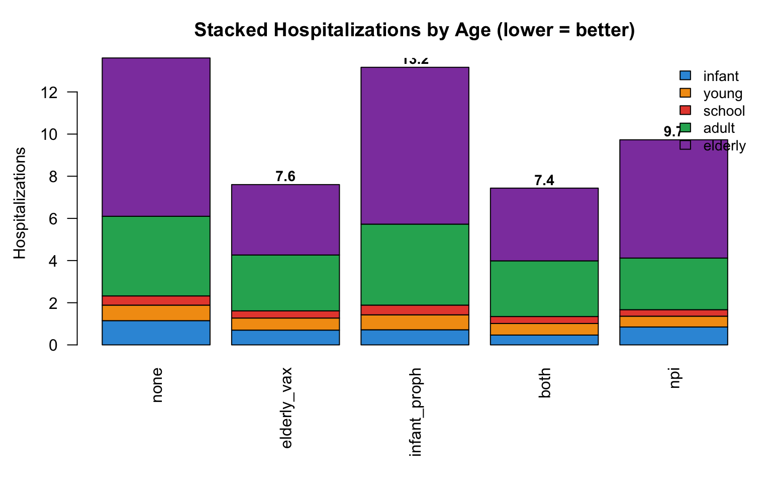
Hospitalizations averted, with uncertainty
Each scenario is compared with the baseline on the per-simulation hospitalization counts, and every difference carries a 95% Monte Carlo interval from the between-simulation variance of the two arms. Averted hospitalizations and the NNI are computed within the age groups each strategy is designed to protect (older adults for the vaccine, infants for the antibody, for the cocoon, and for its random comparator, both for the combined arm, all ages for the NPI), and the all-ages difference is reported next to them with its own interval. The two columns together show why the target-group version is the one to read for the products: the untargeted strata are large, their between-simulation noise is comparable to a product’s whole effect, and the all-ages intervals are correspondingly wide. NNI is reported only when the point estimate of averted hospitalizations is positive, and with an interval only when the whole interval for averted hospitalizations is positive.
mc_diff <- function(x0, x1) {
  d <- mean(x0) - mean(x1)
  if (length(x0) < 2 || length(x1) < 2) return(c(est = d, lo = NA, hi = NA))
  se <- sqrt(var(x0) / length(x0) + var(x1) / length(x1))
  c(est = d, lo = d - 1.96 * se, hi = d + 1.96 * se)
}
fmt_ci <- function(v, digits = 1) {
  if (is.na(v["lo"])) return(sprintf("%.*f", digits, v["est"]))
  sprintf("%.*f (%.*f, %.*f)", digits, v["est"], digits, v["lo"], digits, v["hi"])
}

target_groups <- list(none = age_groups, elderly_vax = "elderly",
                      infant_proph = "infant", both = c("infant", "elderly"),
                      cocoon = "infant", cocoon_random = "infant",
                      npi = age_groups)
per100k <- function(r, groups) 1e5 * rowSums(r$hosp_sim[, groups, drop = FALSE]) / N
averted <- lapply(names(res), function(s) {
  tg <- target_groups[[s]]
  list(target = mc_diff(per100k(res$none, tg), per100k(res[[s]], tg)),
       all = mc_diff(per100k(res$none, age_groups), per100k(res[[s]], age_groups)),
       base_target = mean(per100k(res$none, tg)))
})
names(averted) <- names(res)

nni_of <- function(s) {
  a <- averted[[s]]$target
  doses <- res[[s]]$doses
  averted_n <- a * N / 1e5                  # per 100,000 -> count in N
  if (doses == 0 || is.na(averted_n["est"]) || averted_n["est"] <= 0) return(NA_character_)
  est <- doses / averted_n["est"]
  if (is.na(averted_n["lo"]) || averted_n["lo"] <= 0) {
    return(sprintf("%.0f", est))
  }
  sprintf("%.0f (%.0f, %.0f)", est, doses / averted_n["hi"], doses / averted_n["lo"])
}

int_tbl <- data.frame(
  Scenario = labels[names(res)],
  `Target group` = sapply(names(res), function(s)
    if (length(target_groups[[s]]) == 5) "all ages" else
      paste(target_groups[[s]], collapse = " + ")),
  Doses = sapply(res, function(r) round(r$doses)),
  `Averted in target group` = sapply(names(res), function(s) fmt_ci(averted[[s]]$target)),
  `Percent of target-group baseline` = sapply(names(res), function(s) {
    b <- averted[[s]]$base_target
    if (b > 0) round(100 * averted[[s]]$target["est"] / b, 1) else NA
  }),
  `Averted, all ages` = sapply(names(res), function(s) fmt_ci(averted[[s]]$all)),
  NNI = sapply(names(res), nni_of),
  check.names = FALSE, row.names = NULL
)
knitr::kable(int_tbl,
caption = "Hospitalizations averted relative to no intervention, per 100,000 total population, in the target group and in all ages (95% Monte Carlo intervals in parentheses); doses delivered; and number needed to immunize (doses per hospitalization averted in the target group)")| Scenario | Target group | Doses | Averted in target group | Percent of target-group baseline | Averted, all ages | NNI |
|---|---|---|---|---|---|---|
| No intervention | all ages | 0 | 0.0 (-8.5, 8.5) | 0.0 | 0.0 (-8.5, 8.5) | NA |
| Older-adult vaccine (50%) | elderly | 916 | 20.9 (16.3, 25.5) | 47.5 | 23.9 (15.7, 32.1) | 439 (360, 563) |
| Infant antibody (60%) | infant | 70 | 8.9 (7.4, 10.4) | 44.6 | 13.0 (4.4, 21.5) | 78 (67, 94) |
| Both products | infant + elderly | 959 | 29.8 (24.8, 34.8) | 46.6 | 31.9 (24.4, 39.5) | 322 (276, 387) |
| Household cocoon (all co-residents of infants) | infant | 323 | 3.4 (1.6, 5.3) | 17.3 | 12.4 (2.8, 21.9) | 936 (608, 2034) |
| Same doses, random people of the same ages | infant | 323 | 1.4 (-0.4, 3.3) | 7.2 | 14.4 (3.3, 25.5) | 2243 |
| NPI (days 30-90) | all ages | 0 | 57.1 (49.6, 64.6) | 52.1 | 57.1 (49.6, 64.6) | NA |
scn_int <- setdiff(names(res), "none")
av_est <- sapply(scn_int, function(s) averted[[s]]$target["est"])
av_lo <- sapply(scn_int, function(s) averted[[s]]$target["lo"])
av_hi <- sapply(scn_int, function(s) averted[[s]]$target["hi"])
short <- c(elderly_vax = "Older-adult vaccine", infant_proph = "Infant antibody",
           both = "Both products", cocoon = "Household cocoon",
           cocoon_random = "Random, same doses", npi = "NPI")
par(mfrow = c(1, 2), mar = c(9, 5, 3, 1), mgp = c(3.5, 1, 0))
yr <- range(c(0, av_est, av_lo, av_hi), na.rm = TRUE)
bp2 <- barplot(av_est, names.arg = short[scn_int], col = cols_scn[scn_int],
               las = 2, cex.names = 0.8,
               ylab = "Averted per 100,000 population",
               main = "Averted in Target Groups",
               ylim = yr + diff(yr) * c(-0.05, 0.15))
abline(h = 0)
if (!all(is.na(av_lo))) {
  arrows(bp2, av_lo, bp2, av_hi, angle = 90, code = 3, length = 0.04)
}
text(bp2, pmax(av_hi, av_est, na.rm = TRUE) + diff(yr) * 0.04,
     sprintf("%.1f", av_est), cex = 0.85, font = 2)
nni_num <- sapply(scn_int, function(s) {
  a <- averted[[s]]$target["est"] * N / 1e5
  if (res[[s]]$doses > 0 && !is.na(a) && a > 0) res[[s]]$doses / a else NA
})
keep <- which(!is.na(nni_num))
if (length(keep) > 0) {
  bp3 <- barplot(nni_num[keep], names.arg = short[scn_int[keep]],
                 col = cols_scn[scn_int[keep]], las = 2, cex.names = 0.8,
                 ylab = "Doses per hospitalization averted",
                 main = "Number Needed to Immunize",
                 ylim = c(0, max(nni_num[keep]) * 1.25))
  text(bp3, nni_num[keep] + max(nni_num[keep]) * 0.05,
       sprintf("%.0f", nni_num[keep]), cex = 0.85, font = 2)
}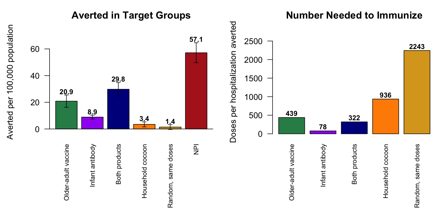
Two features of these results carry over to the published scenario models. First, the older-adult vaccine averts the most hospitalizations in absolute terms because older adults are a large group with a high per-infection risk, while the infant antibody is the more efficient product per dose (an NNI of 78 (67, 94) against 439 (360, 563) here) because infants have the highest per-infection risk but are about 1% of the population. Second, the two products are close to additive, since they act on different people. The cocoon rows are the ones to read with their intervals. Even a complete household cocoon averts 3.4 (1.6, 5.3) infant hospitalizations per 100,000, 17.3% of the infant baseline, at an NNI of 936 (608, 2034), many times the infant antibody’s. The random arm, with the same doses to the same ages, averts 1.4 (-0.4, 3.3), an interval that includes zero, so most of the cocoon’s infant effect comes from the household link rather than from immunizing that many people. Both arms also lower the all-ages total by a similar and imprecisely estimated amount, which is the indirect effect of giving several hundred people, including children, a transmission-blocking product.
Realized product effectiveness
The 80% effectiveness against hospitalization is an input per exposure. What a recipient experiences over a season depends on how often they are exposed, because the infection-blocking component is leaky. The realized effectiveness against infection among recipients is one minus the ratio of the attack rate among immunized to that among unimmunized members of the same group in the same scenario, and the realized effectiveness against hospitalization follows from it and the severity component.
ve_tbl <- do.call(rbind, lapply(c("elderly_vax", "infant_proph"), function(s) {
  a <- if (s == "elderly_vax") "elderly" else "infant"
  r <- res[[s]]
  ve_inf <- ifelse(r$attack_unprot[, a] > 0,
                   1 - r$attack_prot[, a] / r$attack_unprot[, a], NA)
  ve_hosp <- 1 - (1 - ve_inf) * (1 - eff_hosp[a])
  ci <- function(v) {
    m <- mean(v, na.rm = TRUE)
    if (sum(!is.na(v)) < 2) return(sprintf("%.0f", 100 * m))
    se <- sd(v, na.rm = TRUE) / sqrt(sum(!is.na(v)))
    sprintf("%.0f (%.0f, %.0f)", 100 * m, 100 * (m - 1.96 * se), 100 * (m + 1.96 * se))
  }
  eff_inf <- if (a == "elderly") param_base$elderly.vax.eff.inf else param_base$infant.proph.eff.inf
  data.frame(Product = labels[s], Group = a,
             `eff.inf (per contact)` = 100 * eff_inf,
             `Realized VE, infection` = ci(ve_inf),
             `eff.hosp` = 100 * eff_hosp[a],
             `VE, hospitalization, per exposure` = round(100 * (1 - (1 - eff_inf) * (1 - eff_hosp[a]))),
             `Realized VE, hospitalization` = ci(ve_hosp),
             check.names = FALSE, row.names = NULL)
}))
knitr::kable(ve_tbl,
caption = "Product effectiveness among recipients (%): the per-contact and per-exposure inputs, and the realized season-long values from the simulation (95% Monte Carlo intervals in parentheses)")| Product | Group | eff.inf (per contact) | Realized VE, infection | eff.hosp | VE, hospitalization, per exposure | Realized VE, hospitalization |
|---|---|---|---|---|---|---|
| Older-adult vaccine (50%) | elderly | 50 | 45 (32, 58) | 60 | 80 | 78 (73, 83) |
| Infant antibody (60%) | infant | 30 | 6 (-2, 14) | 71 | 80 | 73 (70, 75) |
For older adults, who are exposed rarely, the realized effectiveness against infection is close to the per-contact input and the realized effectiveness against hospitalization is close to the 80% assumed. For infants, who are exposed repeatedly at home, the leaky component protects little over the season (6% against infection from a per-contact input of 30%), and the realized effectiveness against hospitalization is 73% rather than 80%. A model that wants the Hub’s 80% to hold at the season level for infants should either put more of the effect into the severity component or use an all-or-nothing infection-blocking component.
Indirect effects
The indirect effect of each strategy is read from the attack rate among people who did not receive it, with a Monte Carlo interval:
unprot_tbl <- sapply(res, function(r) sapply(c("infant", "elderly"), function(a) {
  v <- 100 * r$attack_unprot[, a]
  if (length(v) < 2) return(sprintf("%.1f", mean(v)))
  se <- sd(v) / sqrt(length(v))
  sprintf("%.1f (%.1f, %.1f)", mean(v), mean(v) - 1.96 * se, mean(v) + 1.96 * se)
}))
knitr::kable(unprot_tbl,
caption = "Cumulative attack rate (%) among unimmunized infants and older adults, by scenario, mean of simulations (95% Monte Carlo intervals in parentheses)")| none | elderly_vax | infant_proph | both | cocoon | cocoon_random | npi | |
|---|---|---|---|---|---|---|---|
| infant | 56.8 (53.8, 59.9) | 53.8 (50.2, 57.5) | 55.5 (50.4, 60.6) | 54.0 (48.1, 60.0) | 47.0 (42.7, 51.4) | 52.7 (48.6, 56.9) | 28.0 (23.7, 32.4) |
| elderly | 5.4 (4.9, 5.8) | 4.7 (4.1, 5.3) | 5.1 (4.6, 5.5) | 4.6 (4.0, 5.2) | 4.9 (4.4, 5.3) | 4.4 (3.7, 5.2) | 2.6 (2.2, 2.9) |
Neither product moves the attack rate among the unimmunized members of its own group by more than the intervals allow, because neither infants nor older adults drive transmission: the infection-blocking component eff.inf removes few transmission chains. With 10 simulations the intervals rule out large indirect effects but not small ones, which is the honest statement of this result; compartmental RSV models produce the same qualitative finding, and it is why the products are usually evaluated on direct protection alone. The NPI lowers both rows because it acts on the children who feed infections into every other group.
The household cocoon is the mirror image: no infant is immunized, so its whole infant effect is indirect, obtained by blocking the household ties through which infants are infected. The per-layer infection counts show why that effect is limited even at complete coverage:
knitr::kable(t(sapply(res, function(r) round(100 * r$hh_share_infant, 1))),
caption = "Share of infant infections acquired from household contacts (%), by scenario")About 40% of infant infections come from the household, and the cocoon acts only on that share, through a leaky 50% reduction in the co-residents’ own per-contact susceptibility, which protects them by less than 50% over a season of repeated exposure. The remaining exposure is in the community layer, where infants have few contacts but full susceptibility. Every cocooning dose also goes to someone whose own hospitalization risk is low, so the NNI is far worse than the direct product’s. The same ordering, direct product over cocooning for severe infant outcomes, appears in household-structured RSV models built for policy.
Who infects whom
Every transmission in every simulation was recorded with set_transmat(), and get_transmat() returns one table per simulation with the extra columns the module added. Pooled over the baseline simulations, the records give the age-by-age transmission matrix, the layer split, and an estimate of the reproduction number: the mean number of secondary infections generated by the seed infections, which were placed at random across ages into a fully susceptible population.
tm_none <- do.call(rbind, lapply(seq_len(nsims), function(s) {
  as.data.frame(get_transmat(sims$none, sim = s))
}))
tm_none$infAge <- factor(tm_none$infAge, levels = age_groups)
tm_none$susAge <- factor(tm_none$susAge, levels = age_groups)
waifw <- round(100 * prop.table(table(infector = tm_none$infAge,
                                      recipient = tm_none$susAge)), 1)
knitr::kable(waifw,
caption = "Who infects whom: percent of all baseline infections by infector age group (rows) and recipient age group (columns), pooled over simulations")| infant | young | school | adult | elderly | |
|---|---|---|---|---|---|
| infant | 0.6 | 1.0 | 0.6 | 1.6 | 0.1 |
| young | 2.3 | 13.9 | 3.0 | 8.7 | 1.1 |
| school | 0.6 | 2.2 | 22.2 | 11.9 | 1.4 |
| adult | 0.8 | 3.4 | 6.6 | 12.6 | 1.9 |
| elderly | 0.1 | 0.3 | 0.3 | 0.9 | 2.0 |
caused <- round(100 * prop.table(table(tm_none$infAge)), 1)
hh_layer <- round(100 * mean(tm_none$layer == 1), 1)
n_seeds <- round(0.01 * N)
r_seed <- round(sum(tm_none$infTime == 1) / (n_seeds * nsims), 2)
c(share_household_layer = hh_layer, secondary_infections_per_seed = r_seed)
share_household_layer secondary_infections_per_seed
44.70 1.17 School-age children cause 38.3% of infections and young children 29%, against 23% of the population between them, and 44.7% of all transmission happens inside households. The seed infections each generated 1.17 secondary infections on average. That number is a reproduction number for a randomly placed infector in a fully susceptible population at the seasonal peak, and it is only modestly above one: the epidemic grows because children, who are contacted and infected more than the average seed, sustain it, and it ends as the seasonal forcing brings transmissibility down and the susceptible children are depleted.
inf_tm <- tm_none[tm_none$susAge == "infant", ]
infant_src <- round(100 * prop.table(table(
  infector = inf_tm$infAge,
  layer = factor(inf_tm$layer, levels = 1:2, labels = c("household", "community")))), 1)
knitr::kable(infant_src,
caption = "Infant infections by infector age group and layer, percent of all infant infections in the baseline simulations")| household | community | |
|---|---|---|
| infant | 0.0 | 14.1 |
| young | 23.9 | 29.8 |
| school | 8.3 | 4.7 |
| adult | 8.9 | 9.0 |
| elderly | 0.3 | 1.1 |
This table is the model’s answer to the pathway question. In a rural Kenyan household cohort, 54% of infant infections were acquired within the household and school-age siblings were the index case for most of those (Munywoki et al. 2014); that setting has larger households and less child care than the one modeled here, and the split is not universal. In this model the household share of infant infections is 41% and the largest single source is young children, at home and in child care. Changing the household mix or the infant entries of the contact profile moves this table directly, which is the point of having it.
Between-simulation variability
hosp_total_sims <- do.call(cbind, lapply(res, function(r) per100k(r, age_groups)))
knitr::kable(round(rbind(mean = colMeans(hosp_total_sims),
                         min = apply(hosp_total_sims, 2, min),
                         max = apply(hosp_total_sims, 2, max))),
caption = "All-ages hospitalizations per 100,000: mean and range across simulations")| none | elderly_vax | infant_proph | both | cocoon | cocoon_random | npi | |
|---|---|---|---|---|---|---|---|
| mean | 110 | 86 | 97 | 78 | 97 | 95 | 53 |
| min | 92 | 70 | 79 | 65 | 75 | 68 | 38 |
| max | 124 | 100 | 116 | 89 | 115 | 116 | 62 |
df_none <- as.data.frame(sims$none)
last_none <- df_none[df_none$time == max(df_none$time), ]
cv <- sapply(age_groups, function(a) {
  v <- last_none[[paste0("cuminf.", a)]]; sd(v) / mean(v)
})
round(cv, 2)
infant young school adult elderly
0.09 0.09 0.14 0.10 0.14 A stochastic epidemic that grows only modestly on a clustered network has a wide final-size distribution even with seasonal forcing, and the small strata at the age extremes add sampling noise on top. The coefficient of variation of season-end infections across the 10 baseline simulations is about 0.1 in every age group, so the standard error of a scenario mean is a few percent of its value. That is small next to the 40% reductions the products produce in their own groups and large next to the few-percent movements in untargeted groups, which is why averted hospitalizations are computed within target groups above and why every effect carries an interval. It is also why the example uses N = 10000 rather than the Gallery’s usual 500 to 1500. More simulations narrow the intervals in proportion to the square root of their number; nsims = 5 halves the run time at the cost of intervals about 40% wider.
Next Steps
- Births, infant age in months, and maternal vaccination. Add an arrivals module so infants are born during the season and receive the antibody at birth or at a catch-up visit, and track infant age in months so that maternal antibody, which protects the youngest infants, can be represented. New arrivals must also be wired into an existing household by appending their edges to
hh.pairs, which is the one piece of bookkeeping the static layer needs. See SI with Vital Dynamics for the aging and arrivals pattern. - Contact persistence. Raise
durationindissolution_coefs()for the community layer while holding the profile fixed, so that the same mean degree is made of repeated rather than fresh contacts, and compare the transmission matrix and the household share of infant infections with the daily-replacement version here. - Age-dependent natural history. Give infants a longer and adults a shorter infectious period, and let the asymptomatic fraction rise with age, as household studies of RSV report.
- Weighted household ties. Give parent-infant, sibling-infant, and grandparent-infant pairs different per-contact probabilities, so that household composition rather than only household size shapes who infects infants.
- Waning and multiple seasons. Add R-to-S waning of natural immunity and a decline in product protection between seasons. The older-adult vaccines lose an estimated 20-30% of their effectiveness per year, which changes the second-season NNI substantially.
- Seasonality from data. The cosine forcing here has an illustrative amplitude and starts the run at the peak. Estimate the amplitude and phase from a surveillance time series, or replace the cosine with the school-calendar forcing that RSV transmission models use, and start the run at season onset with a smaller seed.
- Calibration to surveillance data. Fit the transmission probabilities and
sus.multso that the age-specific hospitalization rates match a season of RSV-NET (issue #58). - Exposure-history immunity. Track the number of prior infections per node instead of using age as the proxy, following the structure in Pitzer et al. (2015).
- Cross-layer dependency. The community layer is independent of household membership. See the SISMID Multi-Layer Networks tutorial for a
dat.updatescallback that links degree across layers.
References
CDC guidance and surveillance (accessed September 2026):
- CDC, RSV vaccine guidance for adults: https://www.cdc.gov/rsv/hcp/vaccine-clinical-guidance/adults.html
- CDC, RSV immunization guidance for infants and young children: https://www.cdc.gov/rsv/hcp/vaccine-clinical-guidance/infants-young-children.html
- CDC, RSV Hospitalization Surveillance Network (RSV-NET): https://www.cdc.gov/rsv/php/surveillance/rsv-net.html
Product trials:
- Hammitt LL, Dagan R, Yuan Y, et al. (2022). Nirsevimab for prevention of RSV in healthy late-preterm and term infants. N Engl J Med 386(9):837-846. https://doi.org/10.1056/NEJMoa2110275
- Simões EAF, Madhi SA, Muller WJ, et al. (2023). Efficacy of nirsevimab against respiratory syncytial virus lower respiratory tract infections in preterm and term infants: a pooled analysis of randomised controlled trials. Lancet Child Adolesc Health 7(3):180-189. https://doi.org/10.1016/S2352-4642(22)00321-2
- Papi A, Ison MG, Langley JM, et al. (2023). Respiratory syncytial virus prefusion F protein vaccine in older adults. N Engl J Med 388(7):595-608. https://doi.org/10.1056/NEJMoa2209604
- Walsh EE, Pérez Marc G, Zareba AM, et al. (2023). Efficacy and safety of a bivalent RSV prefusion F vaccine in older adults. N Engl J Med 388(16):1465-1477. https://doi.org/10.1056/NEJMoa2213836
Epidemiology, natural history, and contact structure:
- Glezen WP, Taber LH, Frank AL, Kasel JA. (1986). Risk of primary infection and reinfection with respiratory syncytial virus. Am J Dis Child 140(6):543-546. https://doi.org/10.1001/archpedi.1986.02140200053026
- Hall CB, Douglas RG, Geiman JM. (1976). Respiratory syncytial virus infections in infants: quantitation and duration of shedding. J Pediatr 89(1):11-15. https://doi.org/10.1016/s0022-3476(76)80918-3
- Hall CB, Long CE, Schnabel KC. (2001). Respiratory syncytial virus infections in previously healthy working adults. Clin Infect Dis 33(6):792-796. https://doi.org/10.1086/322657
- Falsey AR, Hennessey PA, Formica MA, Cox C, Walsh EE. (2005). Respiratory syncytial virus infection in elderly and high-risk adults. N Engl J Med 352(17):1749-1759. https://doi.org/10.1056/NEJMoa043951
- Hall CB, Weinberg GA, Iwane MK, et al. (2009). The burden of respiratory syncytial virus infection in young children. N Engl J Med 360(6):588-598. https://doi.org/10.1056/NEJMoa0804877
- Lessler J, Reich NG, Brookmeyer R, Perl TM, Nelson KE, Cummings DAT. (2009). Incubation periods of acute respiratory viral infections: a systematic review. Lancet Infect Dis 9(5):291-300. https://doi.org/10.1016/S1473-3099(09)70069-6
- Munywoki PK, Koech DC, Agoti CN, et al. (2014). The source of respiratory syncytial virus infection in infants: a household cohort study in rural Kenya. J Infect Dis 209(11):1685-1692. https://doi.org/10.1093/infdis/jit828
- Pitzer VE, Viboud C, Alonso WJ, et al. (2015). Environmental drivers of the spatiotemporal dynamics of respiratory syncytial virus in the United States. PLoS Pathog 11(1):e1004591. https://doi.org/10.1371/journal.ppat.1004591
- Mossong J, Hens N, Jit M, et al. (2008). Social contacts and mixing patterns relevant to the spread of infectious diseases. PLoS Med 5(3):e74. https://doi.org/10.1371/journal.pmed.0050074
RSV scenario modeling tools:
- RSV Scenario Modeling Hub: https://rsvscenariomodelinghub.org/ (Round 4 scenario definitions and intervention effectiveness, accessed September 2026: https://github.com/midas-network/rsv-scenario-modeling-hub)
- Hansen CL, et al. R.Scenario.Vax: scenario projections of RSV hospitalizations from RSV-NET data. https://chelsea-hansen.github.io/R.Scenario.Vax/
- Hansen CL, et al. (2025). Scenario projections of respiratory syncytial virus hospitalizations averted due to new immunizations. JAMA Netw Open 8(6):e2514622. https://doi.org/10.1001/jamanetworkopen.2025.14622
The household mix, community contact profile, per-contact transmission probabilities, susceptibility multipliers, and per-infection hospitalization risks are illustrative choices selected to reproduce the qualitative RSV pattern (attack rates decreasing with age after early childhood, hospitalization burden at the age extremes, children as the transmission amplifier). They are not calibrated to any surveillance dataset or season.