flowchart TD
    in(( )) -->|"arrival<br/>(+/- protection)"| S

    S["<b>S</b><br/>Susceptible<br/><i>protected: reduced FOI</i>"] -->|"infection<br/>(se.flow)"| E["<b>E</b><br/>Exposed"]
    E -->|"progression<br/>(ei.rate)"| I["<b>I</b><br/>Infectious"]
    I -->|"recovery<br/>(ir.rate)"| R["<b>R</b><br/>Recovered"]
    R -->|"waning immunity<br/>(rs.rate)"| S

    S -->|"departure"| out1(( ))
    E -->|"departure"| out2(( ))
    I -->|"departure<br/>(elevated)"| out3(( ))
    R -->|"departure"| out4(( ))

    style S fill:#3498db,color:#fff
    style E fill:#f39c12,color:#fff
    style I fill:#e74c3c,color:#fff
    style R fill:#27ae60,color:#fff
    style in fill:none,stroke:none
    style out1 fill:none,stroke:none
    style out2 fill:none,stroke:none
    style out3 fill:none,stroke:none
    style out4 fill:none,stroke:none
SEIRS with Leaky Vaccination
SEIRS
vaccination
vaccine efficacy
vital dynamics
intermediate
Implements leaky vaccination where protection reduces (rather than eliminates) infection risk, on an SEIRS model with waning immunity and vital dynamics.
Overview
This example demonstrates how to model a leaky vaccination intervention on an SEIRS epidemic over a dynamic network with vital dynamics (arrivals and departures). In a leaky vaccine model, protected individuals are not fully immune — instead, they face a reduced probability of infection determined by the vaccine efficacy parameter. This contrasts with the all-or-nothing (AON) model where protected individuals are completely immune to infection.
Leaky vaccines are the more realistic model for many real-world vaccines (e.g., influenza, pertussis, COVID-19) where protection reduces the likelihood of infection but does not eliminate it. The key parameter is vaccine.efficacy (\(\psi\)): a protected individual’s transmission probability is reduced to \((1 - \psi) \times\) inf.prob. With 80% efficacy, a protected individual faces only 20% of the baseline transmission risk per act.
This example also uses a SEIRS disease model with waning natural immunity (R \(\rightarrow\) S), creating endemic dynamics where the disease persists indefinitely. Importantly, vaccine protection persists through the SEIRS cycle: if a protected individual is infected, progresses through E \(\rightarrow\) I \(\rightarrow\) R \(\rightarrow\) S, they retain their protection attribute and benefit from reduced transmission probability again upon re-entering the susceptible pool.
TipDownload the Standalone Scripts
If you prefer working with standalone R scripts rather than this annotated walkthrough, you can download the original files:
- model.R — Main simulation script
- module-fx.R — Custom module functions
Model Structure
The SEIRS model uses four disease compartments. Unlike the AON vaccination model, there is no separate “V” compartment — vaccine-protected individuals remain in the susceptible compartment with a reduced force of infection.
| Compartment | Label | Description |
|---|---|---|
| Susceptible | S | Not infected; at risk (includes vaccine-protected with reduced FOI) |
| Exposed | E | Infected but not yet infectious (latent period) |
| Infectious | I | Infected and capable of transmitting |
| Recovered | R | Recovered with temporary natural immunity |
The leaky vaccine modifies the infection module rather than using a separate compartment. For each discordant edge, the infection module checks whether the susceptible partner has vaccine protection. If protected, the per-act transmission probability is reduced to \((1 - \psi) \times\) inf.prob; if unprotected, the full inf.prob applies. The per-timestep probability is then computed as \(1 - (1 - \text{transProb})^{\text{act.rate}}\).
AON vs. Leaky Comparison
Understanding the distinction between all-or-nothing and leaky vaccine models is central to this example. The table below summarizes the key differences.
| Feature | All-or-Nothing | Leaky |
|---|---|---|
| Protection type | Complete immunity | Reduced transmission probability |
| Compartment | Separate V compartment | Remains in S |
| Breakthrough infections | Impossible for protected | Possible at reduced rate |
| Implementation | Exclude from discordant edgelist | Modify transProb per edge |
| Disease model | SEIR (permanent immunity) | SEIRS (waning immunity) |
Setup
We begin by loading EpiModel and setting the simulation parameters. The interactive values below are suitable for exploratory analysis; the standalone model.R script uses smaller values for automated testing.
library(EpiModel)

nsims <- 5
ncores <- 5
nsteps <- 500
Custom Modules
This model requires four custom module functions: infection with leaky vaccine protection, SEIRS disease progression, departures with disease-induced excess mortality, and arrivals with a three-route vaccination cascade.
Infection Module
The infection module replaces EpiModel’s built-in transmission function to implement heterogeneous transmission probabilities based on vaccine protection status. For each discordant edge (an S-I partnership), the module checks whether the susceptible partner has vaccine protection. Protected susceptibles face a reduced transmission probability; unprotected susceptibles face the full baseline probability.
infect <- function(dat, at) {

  ## Attributes ##
  active <- get_attr(dat, "active")
  status <- get_attr(dat, "status")
  infTime <- get_attr(dat, "infTime")
  protection <- get_attr(dat, "protection")

  ## Parameters ##
  inf.prob <- get_param(dat, "inf.prob")
  act.rate <- get_param(dat, "act.rate")
  vaccine.efficacy <- get_param(dat, "vaccine.efficacy")

  ## Find infected nodes ##
  idsInf <- which(active == 1 & status == "i")
  nActive <- sum(active == 1)
  nElig <- length(idsInf)

  ## Initialize incidence counter ##
  nInf <- 0

  ## Transmission process ##
  if (nElig > 0 && nElig < nActive) {

    del <- discord_edgelist(dat, at)

    if (!(is.null(del))) {

1      inf.prob.reduced <- (1 - vaccine.efficacy) * inf.prob
      idsProtected <- which(
        !is.na(protection) & protection != "none" &
          status == "s" & active == 1
      )

      protDF <- data.frame(
        sus = idsProtected,
        transProb = rep(inf.prob.reduced, length(idsProtected))
      )
2      del <- merge(del, protDF, by = "sus", all.x = TRUE)

3      del$transProb <- ifelse(is.na(del$transProb), inf.prob, del$transProb)

      del$actRate <- act.rate
4      del$finalProb <- 1 - (1 - del$transProb)^del$actRate

      transmit <- rbinom(nrow(del), 1, del$finalProb)
      del <- del[which(transmit == 1), ]

      idsNewInf <- unique(del$sus)
      nInf <- length(idsNewInf)

      if (nInf > 0) {
5        status[idsNewInf] <- "e"
        dat <- set_attr(dat, "status", status)
        infTime[idsNewInf] <- at
        dat <- set_attr(dat, "infTime", infTime)
      }
    }
  }

  ## Summary statistics ##
  dat <- set_epi(dat, "se.flow", at, nInf)

  dat <- set_epi(dat, "s.num", at, sum(active == 1 & status == "s"))
  dat <- set_epi(dat, "e.num", at, sum(active == 1 & status == "e"))
  dat <- set_epi(dat, "i.num", at, sum(active == 1 & status == "i"))
  dat <- set_epi(dat, "r.num", at, sum(active == 1 & status == "r"))

  return(dat)
}- 1
-
Compute the reduced transmission probability for protected individuals: \((1 - \psi) \times\)
inf.prob. - 2
- Merge the protection lookup onto the discordant edgelist so each edge knows its susceptible partner’s protection status.
- 3
-
Unprotected susceptibles (no match in the merge) get the full
inf.prob. - 4
- Convert the per-act probability to a per-timestep probability accounting for multiple acts: \(1 - (1 - p)^a\).
- 5
- Newly infected individuals enter the Exposed (E) compartment, not directly Infectious.
Disease Progression Module
The progression module handles the three disease transitions in the SEIRS cycle: E \(\rightarrow\) I (latent to infectious), I \(\rightarrow\) R (infectious to recovered), and R \(\rightarrow\) S (waning natural immunity). The R \(\rightarrow\) S transition is what creates endemic dynamics — recovered individuals eventually return to the susceptible pool and can be reinfected. Crucially, if a vaccine-protected individual cycles through the entire SEIRS pathway, they retain their protection attribute and benefit from reduced transmission probability upon re-entering S.
progress <- function(dat, at) {

  ## Attributes ##
  active <- get_attr(dat, "active")
  status <- get_attr(dat, "status")

  ## Parameters ##
  ei.rate <- get_param(dat, "ei.rate")
  ir.rate <- get_param(dat, "ir.rate")
  rs.rate <- get_param(dat, "rs.rate")

  ## E -> I (exposed to infectious) ##
  nProg <- 0
  idsEligProg <- which(active == 1 & status == "e")
  nEligProg <- length(idsEligProg)

  if (nEligProg > 0) {
    vecProg <- which(rbinom(nEligProg, 1, ei.rate) == 1)
    if (length(vecProg) > 0) {
      idsProg <- idsEligProg[vecProg]
      nProg <- length(idsProg)
      status[idsProg] <- "i"
    }
  }

  ## I -> R (infectious to recovered) ##
  nRec <- 0
  idsEligRec <- which(active == 1 & status == "i")
  nEligRec <- length(idsEligRec)

  if (nEligRec > 0) {
    vecRec <- which(rbinom(nEligRec, 1, ir.rate) == 1)
    if (length(vecRec) > 0) {
      idsRec <- idsEligRec[vecRec]
      nRec <- length(idsRec)
      status[idsRec] <- "r"
    }
  }

  ## R -> S (recovered to susceptible, waning immunity) ##
  nSus <- 0
  idsEligSus <- which(active == 1 & status == "r")
  nEligSus <- length(idsEligSus)

  if (nEligSus > 0) {
1    vecSus <- which(rbinom(nEligSus, 1, rs.rate) == 1)
    if (length(vecSus) > 0) {
      idsSus <- idsEligSus[vecSus]
      nSus <- length(idsSus)
2      status[idsSus] <- "s"
    }
  }

  ## Write out updated status ##
  dat <- set_attr(dat, "status", status)

  ## Summary statistics ##
  dat <- set_epi(dat, "ei.flow", at, nProg)
  dat <- set_epi(dat, "ir.flow", at, nRec)
  dat <- set_epi(dat, "rs.flow", at, nSus)

  return(dat)
}- 1
-
Waning immunity is stochastic: each recovered individual independently loses immunity at rate
rs.rateper timestep. - 2
-
Individuals returning to S retain any vaccine protection attribute — the module only changes
status, notprotection.
Departure Module
The departure module simulates mortality with disease-induced excess. All active nodes face a baseline departure.rate per timestep. Infected individuals (status = “i”) face an elevated rate multiplied by departure.disease.mult, representing excess disease-induced mortality.
dfunc <- function(dat, at) {

  ## Attributes ##
  active <- get_attr(dat, "active")
  status <- get_attr(dat, "status")
  exitTime <- get_attr(dat, "exitTime")

  ## Parameters ##
  departure.rate <- get_param(dat, "departure.rate")
  departure.rates <- rep(departure.rate, length(active))
  departure.dis.mult <- get_param(dat, "departure.disease.mult")

  ## Determine eligible (alive) nodes ##
  idsElig <- which(active == 1)
  nElig <- length(idsElig)
  nDepartures <- 0

  if (nElig > 0) {

    dep_rates_of_elig <- departure.rates[idsElig]

    idsElig.inf <- which(status[idsElig] == "i")
    dep_rates_of_elig[idsElig.inf] <- departure.rates[idsElig.inf] *
1      departure.dis.mult

    ## Stochastic departure process ##
    vecDeparture <- which(rbinom(nElig, 1, dep_rates_of_elig) == 1)
    idsDeparture <- idsElig[vecDeparture]
    nDepartures <- length(idsDeparture)

    if (nDepartures > 0) {
2      active[idsDeparture] <- 0
      exitTime[idsDeparture] <- at
    }
  }

  ## Write out updated attributes ##
  dat <- set_attr(dat, "active", active)
  dat <- set_attr(dat, "exitTime", exitTime)

  ## Summary statistics ##
  dat <- set_epi(dat, "d.flow", at, nDepartures)

  return(dat)
}- 1
-
Infected individuals face
departure.rate * departure.disease.mult(2x the baseline), representing disease-induced excess mortality. - 2
-
Setting
active = 0marks the node as departed; EpiModel handles network dissolution for inactive nodes.
Arrival Module with Vaccination
The arrival module is the most complex custom function in this example. It handles new node arrivals (births) and implements the full three-route vaccination cascade. The three routes are: (1) initialization of the starting population at timestep 2, (2) ongoing vaccination campaigns for unvaccinated nodes, and (3) vaccination of new arrivals at birth. In the leaky model, vaccination confers a protection attribute that reduces transmission probability rather than granting full immunity. Protection persists through the SEIRS cycle, so a protected individual who is infected and later returns to S retains their protection.
afunc <- function(dat, at) {

  ## Attributes ##
  active <- get_attr(dat, "active")
  status <- get_attr(dat, "status")
  infTime <- get_attr(dat, "infTime")

  ## Parameters ##
  nActive <- sum(active == 1)
  nTotal <- length(active)
  a.rate <- get_param(dat, "arrival.rate")
  vaccination.rate.arrivals <- get_param(dat, "vaccination.rate.arrivals")
  protection.rate.arrivals <- get_param(dat, "protection.rate.arrivals")
  vaccination.rate.init <- get_param(dat, "vaccination.rate.initialization")
  protection.rate.init <- get_param(dat, "protection.rate.initialization")
  vaccination.rate.progression <- get_param(dat, "vaccination.rate.progression")
  protection.rate.progression <- get_param(dat, "protection.rate.progression")

  ## Initialize flow counters ##
  nVax.init <- 0
  nPrt.init <- 0
  nVax.prog <- 0
  nPrt.prog <- 0
  nVax.arrival <- 0
  nPrt.arrival <- 0

  ## --- INITIALIZATION (at == 2 only) --- ##
1  if (at == 2) {

    vaccination <- rep(NA, nTotal)
    protection <- rep(NA, nTotal)
    dat <- set_attr(dat, "vaccination", vaccination)
    dat <- set_attr(dat, "protection", protection)

    vaccination <- get_attr(dat, "vaccination")
    protection <- get_attr(dat, "protection")

    idsEligVacInit <- which(active == 1)
    vecVacInit <- rbinom(length(idsEligVacInit), 1, vaccination.rate.init)
    idsVacInit <- idsEligVacInit[which(vecVacInit == 1)]
    vaccination[idsVacInit] <- "initial"

    idsEligProtInit <- which(vaccination == "initial" & status == "s")
    vecProtInit <- rbinom(length(idsEligProtInit), 1, protection.rate.init)
    idsProtInit <- idsEligProtInit[which(vecProtInit == 1)]
    idsNoProtInit <- setdiff(idsVacInit, idsProtInit)
    protection[idsProtInit] <- "initial"
2    protection[idsNoProtInit] <- "none"

    nVax.init <- length(idsVacInit)
    nPrt.init <- length(idsProtInit)

    dat <- set_attr(dat, "vaccination", vaccination)
    dat <- set_attr(dat, "protection", protection)
  }

  vaccination <- get_attr(dat, "vaccination")
  protection <- get_attr(dat, "protection")

  ## --- VACCINATION PROGRESSION --- ##
  idsEligVacProg <- which(is.na(vaccination) & active == 1)
  vecVacProg <- rbinom(length(idsEligVacProg), 1, vaccination.rate.progression)
  idsVacProg <- idsEligVacProg[which(vecVacProg == 1)]
  vaccination[idsVacProg] <- "progress"

  idsEligProtProg <- which(
    vaccination == "progress" & is.na(protection) & status == "s"
  )
  vecProtProg <- rbinom(length(idsEligProtProg), 1, protection.rate.progression)
  idsProtProg <- idsEligProtProg[which(vecProtProg == 1)]
  idsNoProtProg <- setdiff(idsVacProg, idsProtProg)
  protection[idsProtProg] <- "progress"
  protection[idsNoProtProg] <- "none"

  nVax.prog <- length(idsVacProg)
  nPrt.prog <- length(idsProtProg)

  ## --- ARRIVAL PROCESS --- ##
  nArrivalsExp <- nActive * a.rate
3  nArrivals <- rpois(1, nArrivalsExp)

  if (nArrivals > 0) {
4    dat <- append_core_attr(dat, at, nArrivals)

    newNodes <- (nTotal + 1):(nTotal + nArrivals)
    status <- c(status, rep("s", nArrivals))
    infTime <- c(infTime, rep(NA, nArrivals))
    vaccination <- c(vaccination, rep(NA, nArrivals))
    protection <- c(protection, rep(NA, nArrivals))

    vaccinatedNewArrivals <- rbinom(nArrivals, 1, vaccination.rate.arrivals)
    vaccination[newNodes] <- ifelse(vaccinatedNewArrivals == 1, "arrival", NA)
    nVax.arrival <- sum(vaccinatedNewArrivals == 1)

    idsEligProtArrival <- which(
      vaccination == "arrival" & status == "s" & is.na(protection)
    )
    vecProtArrival <- rbinom(length(idsEligProtArrival), 1,
                             protection.rate.arrivals)
    idsProtArrival <- idsEligProtArrival[which(vecProtArrival == 1)]
    idsNoProtArrival <- idsEligProtArrival[which(vecProtArrival == 0)]
    protection[idsProtArrival] <- "arrival"
    protection[idsNoProtArrival] <- "none"
    nPrt.arrival <- sum(vecProtArrival == 1)
  }

  ## Write out updated attributes ##
  dat <- set_attr(dat, "vaccination", vaccination)
  dat <- set_attr(dat, "protection", protection)
  dat <- set_attr(dat, "infTime", infTime)
  dat <- set_attr(dat, "status", status)

  ## Summary statistics ##
  active <- get_attr(dat, "active")
  dat <- set_epi(dat, "a.flow", at, nArrivals)
  dat <- set_epi(dat, "vac.flow", at, nVax.init + nVax.prog + nVax.arrival)
  dat <- set_epi(dat, "prt.flow", at, nPrt.init + nPrt.prog + nPrt.arrival)
  dat <- set_epi(dat, "vac.num", at,
                 sum(active == 1 & vaccination %in%
                       c("initial", "progress", "arrival"), na.rm = TRUE))
5  dat <- set_epi(dat, "prt.num", at,
                 sum(active == 1 & protection %in%
                       c("initial", "progress", "arrival"), na.rm = TRUE))

  return(dat)
}- 1
-
EpiModel convention: modules first execute at timestep 2 (timestep 1 is reserved for
init.net). Custom attributes likevaccinationandprotectionare initialized here. - 2
-
Vaccinated individuals who do not gain protection are tagged
"none"— they cannot be re-vaccinated, modeling a one-shot vaccination assumption. - 3
- Arrivals are drawn from a Poisson distribution with expectation equal to the current active population times the arrival rate.
- 4
-
append_core_attr()registers the new nodes in EpiModel’s internal data structures (active status, unique IDs, etc.). - 5
-
prt.numtracks the number of actively protected individuals across all three vaccination routes, used in the vaccine coverage plot.
Network Model
We initialize a 500-node network and fit an edges-only ERGM with a mean degree of 0.8 (200 edges). The dissolution coefficient accounts for population turnover so that the observed partnership duration matches the target of 50 weeks.
n <- 500
nw <- network_initialize(n)

formation <- ~edges
mean_degree <- 0.8
n_edges <- mean_degree * (n / 2)
target.stats <- c(n_edges)
departure_rate <- 0.008
coef.diss <- dissolution_coefs(dissolution = ~offset(edges),
1 duration = 50, d.rate = departure_rate)
coef.diss- 1
-
The
d.rateargument adjusts the dissolution coefficient so that partnerships ending due to node departure are not double-counted. Without this correction, observed partnership durations would be shorter than the target.
Dissolution Coefficients
=======================
Dissolution Model: ~offset(edges)
Target Statistics: 50
Crude Coefficient: 3.89182
Mortality/Exit Rate: 0.008
Adjusted Coefficient: 5.485385
est <- netest(nw, formation, target.stats, coef.diss)Network Diagnostics
We simulate the dynamic network forward to verify that the ERGM produces the expected network structure. The diagnostics check that the mean number of edges stays near the target of 200 and that the degree distribution is reasonable.
dx <- netdx(est, nsims = nsims, ncores = ncores, nsteps = nsteps,
            nwstats.formula = ~edges + isolates + degree(0:5))
Network Diagnostics
-----------------------
- Simulating 5 networks
- Calculating formation statisticsprint(dx)EpiModel Network Diagnostics
=======================
Diagnostic Method: Dynamic
Simulations: 5
Time Steps per Sim: 500
Formation Diagnostics
-----------------------
Target Sim Mean Pct Diff Sim SE Z Score SD(Sim Means) SD(Statistic)
edges 200 194.994 -2.503 2.080 -2.407 4.756 13.555
isolates NA 227.516 NA 2.351 NA 4.299 14.950
degree0 NA 227.516 NA 2.351 NA 4.299 14.950
degree1 NA 180.840 NA 1.333 NA 2.143 11.879
degree2 NA 70.134 NA 0.922 NA 2.979 8.622
degree3 NA 17.718 NA 0.447 NA 0.790 4.427
degree4 NA 3.302 NA 0.197 NA 0.514 2.061
degree5 NA 0.430 NA 0.077 NA 0.232 0.755
Duration Diagnostics
-----------------------
Target Sim Mean Pct Diff Sim SE Z Score SD(Sim Means) SD(Statistic)
edges 50 50.253 0.506 0.529 0.478 0.982 3.477
Dissolution Diagnostics
-----------------------
Target Sim Mean Pct Diff Sim SE Z Score SD(Sim Means) SD(Statistic)
edges 0.02 0.02 1.468 0 1.392 0 0.01plot(dx)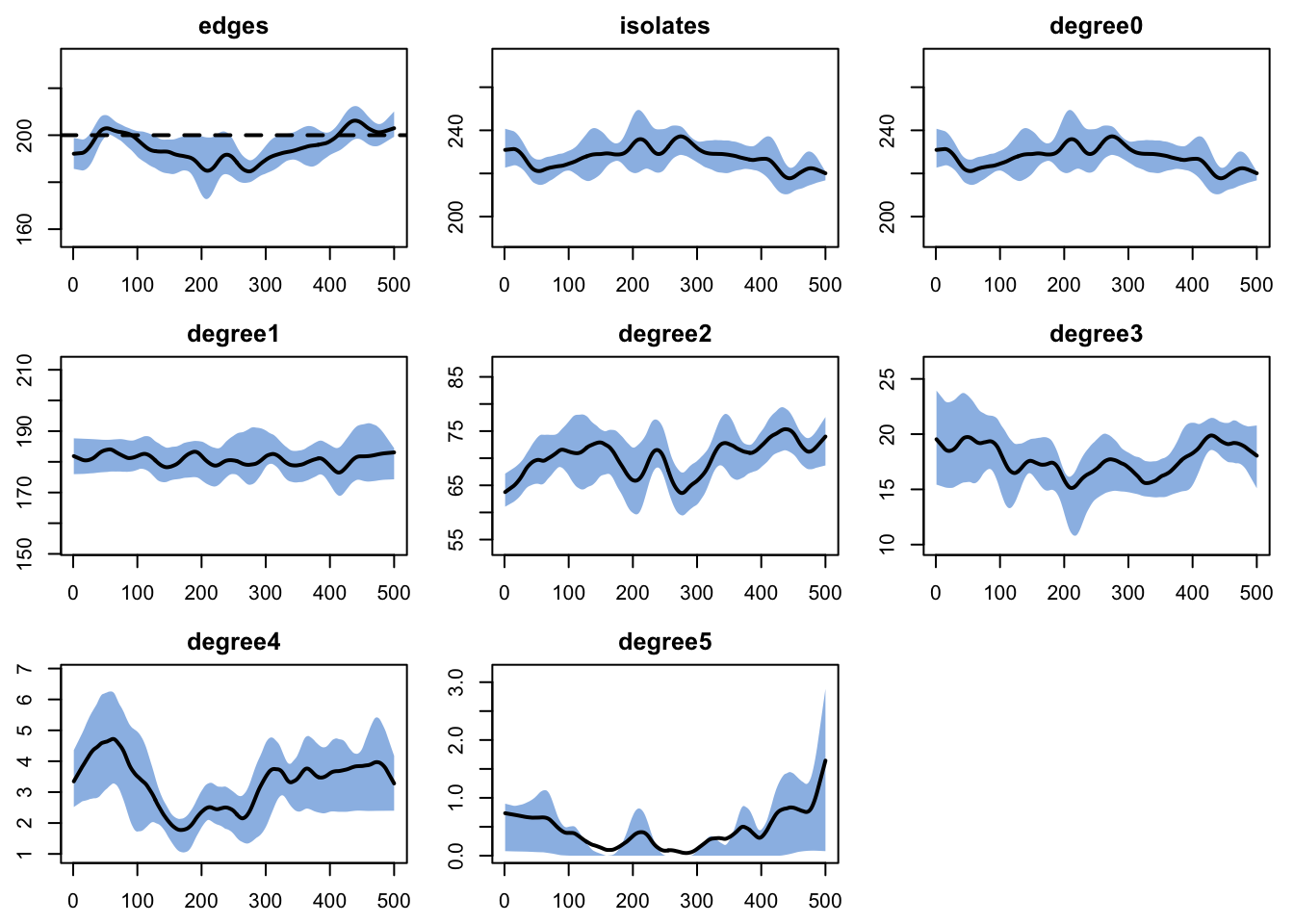
Epidemic Simulation
We run two scenarios to compare the SEIRS epidemic with and without leaky vaccination. Both scenarios use the same network model and initial conditions (20 infected nodes, 4% prevalence).
Initial Conditions and Control Settings
init <- init.net(i.num = 20)control <- control.net(
type = NULL,
nsteps = nsteps,
nsims = nsims,
ncores = ncores,
infection.FUN = infect,
progress.FUN = progress,
departures.FUN = dfunc,
arrivals.FUN = afunc,
1 resimulate.network = TRUE,
verbose = FALSE,
module.order = c("resim_nets.FUN",
"departures.FUN", "arrivals.FUN",
"infection.FUN", "progress.FUN",
2 "prevalence.FUN")
)- 1
-
resimulate.network = TRUEis required because vital dynamics change the population size, so the network must be re-simulated at each timestep. - 2
- The explicit module order ensures departures and arrivals run before infection, so the network reflects the current population when transmission is simulated.
Scenario 1: No Vaccination (SEIRS Baseline)
Without vaccination, the SEIRS model produces endemic dynamics. Waning immunity (R \(\rightarrow\) S at rs.rate) continuously replenishes the susceptible pool, sustaining ongoing transmission indefinitely.
param_novax <- param.net(
  inf.prob = 0.5, act.rate = 1,
  ei.rate = 0.05, ir.rate = 0.05, rs.rate = 0.05,
  departure.rate = departure_rate,
  departure.disease.mult = 2,
  arrival.rate = 0.008,
  vaccination.rate.initialization = 0,
  protection.rate.initialization = 0,
  vaccination.rate.progression = 0,
  protection.rate.progression = 0,
  vaccination.rate.arrivals = 0,
  protection.rate.arrivals = 0,
  vaccine.efficacy = 0
)

sim_novax <- netsim(est, param_novax, init, control)
print(sim_novax)
EpiModel Simulation
=======================
Model class: netsim
Simulation Summary
-----------------------
Model type:
No. simulations: 5
No. time steps: 500
No. NW groups: 1
Fixed Parameters
---------------------------
inf.prob = 0.5
act.rate = 1
ei.rate = 0.05
ir.rate = 0.05
rs.rate = 0.05
departure.rate = 0.008
departure.disease.mult = 2
arrival.rate = 0.008
vaccination.rate.initialization = 0
protection.rate.initialization = 0
vaccination.rate.progression = 0
protection.rate.progression = 0
vaccination.rate.arrivals = 0
protection.rate.arrivals = 0
vaccine.efficacy = 0
groups = 1
Model Functions
-----------------------
initialize.FUN
resim_nets.FUN
summary_nets.FUN
infection.FUN
departures.FUN
arrivals.FUN
nwupdate.FUN
prevalence.FUN
verbose.FUN
progress.FUN
Model Output
-----------------------
Variables: s.num i.num num d.flow a.flow vac.flow prt.flow
vac.num prt.num se.flow e.num r.num ei.flow ir.flow rs.flow
Networks: sim1 ... sim5
Transmissions: sim1 ... sim5
Formation Statistics
-----------------------
Target Sim Mean Pct Diff Sim SE Z Score SD(Sim Means) SD(Statistic)
edges 200 210.2 5.1 Inf 0 16.407 16.407
Duration Statistics
-----------------------
Target Sim Mean Pct Diff Sim SE Z Score SD(Sim Means) SD(Statistic)
edges 50 121.039 142.079 16.058 4.424 2.349 41.046
Dissolution Statistics
-----------------------
Target Sim Mean Pct Diff Sim SE Z Score SD(Sim Means) SD(Statistic)
edges 0.02 0.004 -79.75 0 -305.169 0 0.003Scenario 2: Leaky Vaccination Program
With a leaky vaccine at 80% efficacy, protected individuals face only 20% of the baseline transmission probability. Unlike AON vaccination, protected individuals can still be infected — just at a reduced rate. If infected, they progress through E \(\rightarrow\) I \(\rightarrow\) R \(\rightarrow\) S normally, retaining their protection attribute for subsequent exposures.
param_vax <- param.net(
  inf.prob = 0.5, act.rate = 1,
  ei.rate = 0.05, ir.rate = 0.05, rs.rate = 0.05,
  departure.rate = departure_rate,
  departure.disease.mult = 2,
  arrival.rate = 0.008,
  vaccination.rate.initialization = 0.05,
  protection.rate.initialization = 0.8,
  vaccination.rate.progression = 0.05,
  protection.rate.progression = 0.8,
  vaccination.rate.arrivals = 0.6,
  protection.rate.arrivals = 0.8,
1  vaccine.efficacy = 0.8
)

sim_vax <- netsim(est, param_vax, init, control)
print(sim_vax)- 1
- At 80% efficacy, a protected individual’s per-act transmission probability is reduced from 0.5 to \((1 - 0.8) \times 0.5 = 0.1\).
EpiModel Simulation
=======================
Model class: netsim

Simulation Summary
-----------------------
Model type:
No. simulations: 5
No. time steps: 500
No. NW groups: 1

Fixed Parameters
---------------------------
inf.prob = 0.5
act.rate = 1
ei.rate = 0.05
ir.rate = 0.05
rs.rate = 0.05
departure.rate = 0.008
departure.disease.mult = 2
arrival.rate = 0.008
vaccination.rate.initialization = 0.05
protection.rate.initialization = 0.8
vaccination.rate.progression = 0.05
protection.rate.progression = 0.8
vaccination.rate.arrivals = 0.6
protection.rate.arrivals = 0.8
vaccine.efficacy = 0.8
groups = 1

Model Functions
-----------------------
initialize.FUN
resim_nets.FUN
summary_nets.FUN
infection.FUN
departures.FUN
arrivals.FUN
nwupdate.FUN
prevalence.FUN
verbose.FUN
progress.FUN

Model Output
-----------------------
Variables: s.num i.num num d.flow a.flow vac.flow prt.flow
vac.num prt.num se.flow e.num r.num ei.flow ir.flow rs.flow
Networks: sim1 ... sim5
Transmissions: sim1 ... sim5

Formation Statistics
-----------------------
      Target Sim Mean Pct Diff Sim SE Z Score SD(Sim Means) SD(Statistic)
edges    200    217.6      8.8    Inf       0        16.041        16.041


Duration Statistics
-----------------------
      Target Sim Mean Pct Diff Sim SE Z Score SD(Sim Means) SD(Statistic)
edges     50  122.146  144.292 16.003   4.508         4.268        41.417

Dissolution Statistics
-----------------------
      Target Sim Mean Pct Diff Sim SE  Z Score SD(Sim Means) SD(Statistic)
edges   0.02    0.004  -79.599      0 -289.357             0         0.003
Analysis
We compute derived epidemiological measures and compare the two scenarios visually. The headline result: leaky vaccination reduces but does not eliminate disease. Unlike AON vaccination (which can achieve herd immunity), leaky vaccines allow breakthrough infections, so some transmission persists even at high coverage.
sim_novax <- mutate_epi(sim_novax, prev = i.num / num)
sim_vax <- mutate_epi(sim_vax, prev = i.num / num)
Prevalence Comparison
par(mfrow = c(1, 1), mar = c(3, 3, 2, 1), mgp = c(2, 1, 0))
plot(sim_novax, y = "prev",
     main = "Prevalence: No Vaccination vs. Leaky Vaccination",
     ylab = "Prevalence (I / N)", xlab = "Week",
     mean.col = "firebrick", mean.lwd = 2, mean.smooth = TRUE,
     qnts.col = "firebrick", qnts.alpha = 0.2, qnts.smooth = TRUE,
     legend = FALSE)
plot(sim_vax, y = "prev",
     mean.col = "#27ae60", mean.lwd = 2, mean.smooth = TRUE,
     qnts.col = "#27ae60", qnts.alpha = 0.2, qnts.smooth = TRUE,
     legend = FALSE, add = TRUE)
legend("topright",
       legend = c("No Vaccination", "Leaky Vaccination (80% eff.)"),
       col = c("firebrick", "#27ae60"), lwd = 2, bty = "n")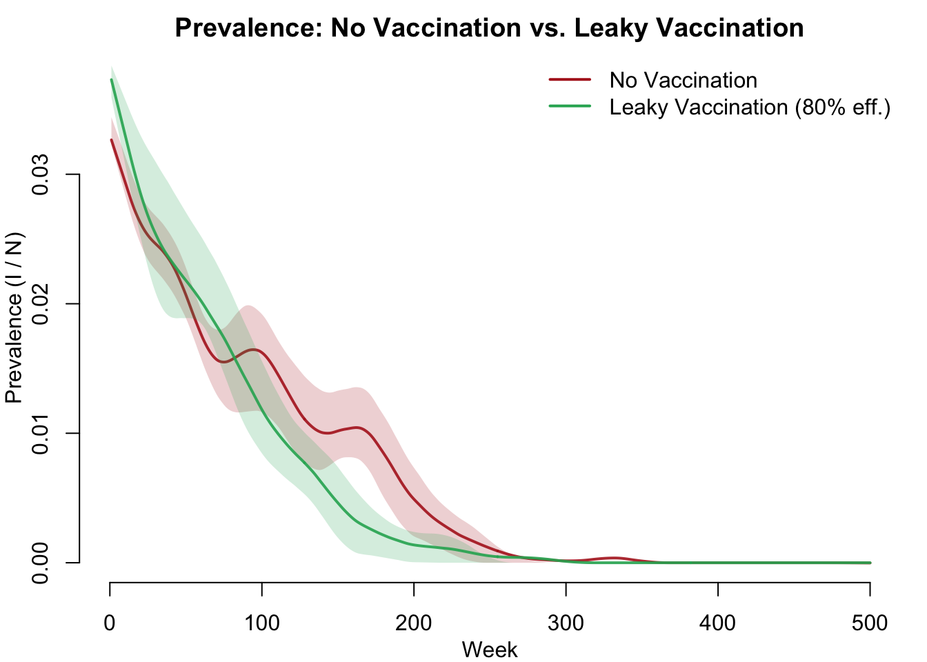
SEIRS Compartments (No Vaccination)
Without vaccination, the SEIRS dynamics show an endemic equilibrium. The R \(\rightarrow\) S waning immunity transition continuously replenishes susceptibles, sustaining ongoing transmission indefinitely.
par(mfrow = c(2, 2), mar = c(3, 3, 2, 1), mgp = c(2, 1, 0))
plot(sim_novax, y = "s.num",
     main = "Susceptible (S)", ylab = "Count", xlab = "Week",
     mean.col = "steelblue", mean.lwd = 2, mean.smooth = TRUE,
     qnts.col = "steelblue", qnts.alpha = 0.2, qnts.smooth = TRUE,
     legend = FALSE)
plot(sim_novax, y = "e.num",
     main = "Exposed (E)", ylab = "Count", xlab = "Week",
     mean.col = "#f39c12", mean.lwd = 2, mean.smooth = TRUE,
     qnts.col = "#f39c12", qnts.alpha = 0.2, qnts.smooth = TRUE,
     legend = FALSE)
plot(sim_novax, y = "i.num",
     main = "Infectious (I)", ylab = "Count", xlab = "Week",
     mean.col = "firebrick", mean.lwd = 2, mean.smooth = TRUE,
     qnts.col = "firebrick", qnts.alpha = 0.2, qnts.smooth = TRUE,
     legend = FALSE)
plot(sim_novax, y = "r.num",
     main = "Recovered (R)", ylab = "Count", xlab = "Week",
     mean.col = "#27ae60", mean.lwd = 2, mean.smooth = TRUE,
     qnts.col = "#27ae60", qnts.alpha = 0.2, qnts.smooth = TRUE,
     legend = FALSE)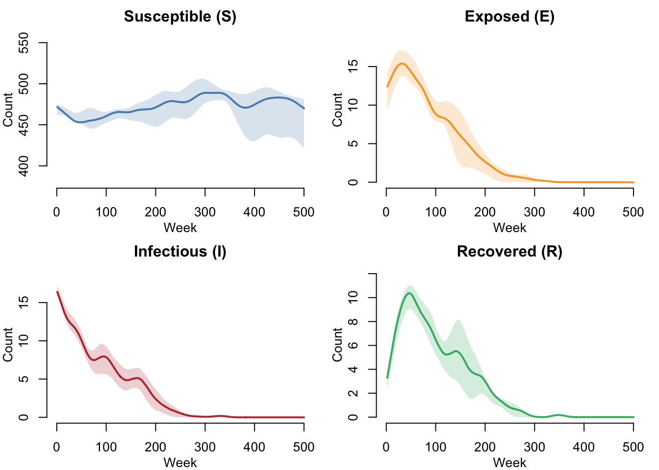
SEIRS Compartments (With Leaky Vaccination)
With vaccination, all disease compartments are reduced as fewer susceptibles become infected. Note that there is no “V” compartment as in the AON model — vaccine-protected individuals remain in S with reduced transmission probability.
par(mfrow = c(2, 2), mar = c(3, 3, 2, 1), mgp = c(2, 1, 0))
plot(sim_vax, y = "s.num",
     main = "Susceptible (S)", ylab = "Count", xlab = "Week",
     mean.col = "steelblue", mean.lwd = 2, mean.smooth = TRUE,
     qnts.col = "steelblue", qnts.alpha = 0.2, qnts.smooth = TRUE,
     legend = FALSE)
plot(sim_vax, y = "e.num",
     main = "Exposed (E)", ylab = "Count", xlab = "Week",
     mean.col = "#f39c12", mean.lwd = 2, mean.smooth = TRUE,
     qnts.col = "#f39c12", qnts.alpha = 0.2, qnts.smooth = TRUE,
     legend = FALSE)
plot(sim_vax, y = "i.num",
     main = "Infectious (I)", ylab = "Count", xlab = "Week",
     mean.col = "firebrick", mean.lwd = 2, mean.smooth = TRUE,
     qnts.col = "firebrick", qnts.alpha = 0.2, qnts.smooth = TRUE,
     legend = FALSE)
plot(sim_vax, y = "r.num",
     main = "Recovered (R)", ylab = "Count", xlab = "Week",
     mean.col = "#27ae60", mean.lwd = 2, mean.smooth = TRUE,
     qnts.col = "#27ae60", qnts.alpha = 0.2, qnts.smooth = TRUE,
     legend = FALSE)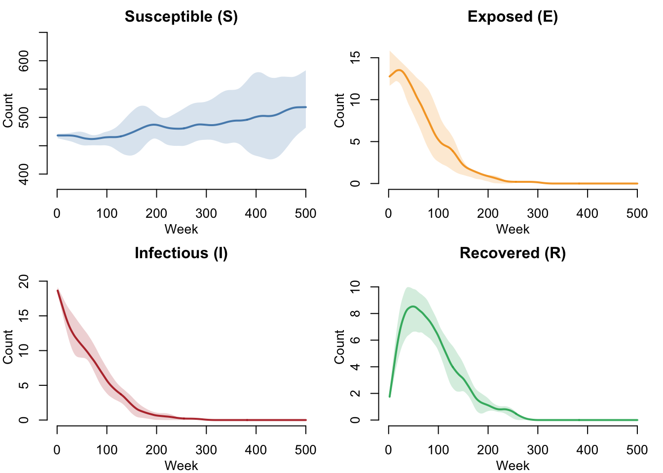
Vaccine Coverage Over Time
The number of active nodes with vaccine protection grows over time as the three vaccination routes accumulate coverage. In the leaky model, these protected individuals are still counted in the S compartment rather than being moved to a separate V compartment.
par(mfrow = c(1, 1), mar = c(3, 3, 2, 1), mgp = c(2, 1, 0))
plot(sim_vax, y = "prt.num",
     main = "Vaccine-Protected Population Over Time",
     ylab = "Protected Individuals", xlab = "Week",
     mean.col = "#8e44ad", mean.lwd = 2, mean.smooth = TRUE,
     qnts.col = "#8e44ad", qnts.alpha = 0.2, qnts.smooth = TRUE,
     legend = FALSE)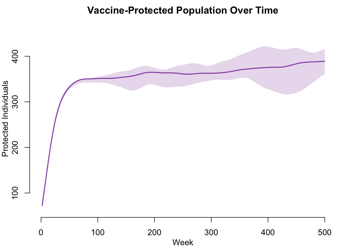
Incidence Comparison
New infections (S \(\rightarrow\) E) per week show the direct impact of leaky vaccination on transmission. Vaccination reduces but does not eliminate new infections — breakthrough infections occur at a reduced rate among protected individuals.
par(mfrow = c(1, 1), mar = c(3, 3, 2, 1), mgp = c(2, 1, 0))
plot(sim_novax, y = "se.flow",
     main = "New Infections per Week",
     ylab = "New Infections (S -> E)", xlab = "Week",
     mean.col = "firebrick", mean.lwd = 2, mean.smooth = TRUE,
     qnts.col = "firebrick", qnts.alpha = 0.2, qnts.smooth = TRUE,
     legend = FALSE)
plot(sim_vax, y = "se.flow",
     mean.col = "#27ae60", mean.lwd = 2, mean.smooth = TRUE,
     qnts.col = "#27ae60", qnts.alpha = 0.2, qnts.smooth = TRUE,
     legend = FALSE, add = TRUE)
legend("topright",
       legend = c("No Vaccination", "Leaky Vaccination (80% eff.)"),
       col = c("firebrick", "#27ae60"), lwd = 2, bty = "n")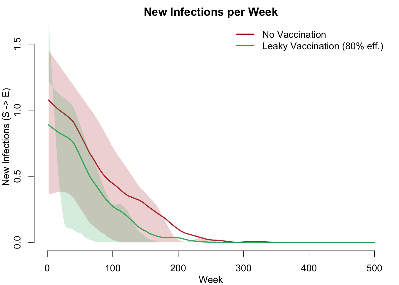
Summary Table
The summary table compares key epidemiological metrics between the two scenarios using the final 20% of the simulation (after transients have settled).
df_novax <- as.data.frame(sim_novax)
df_vax <- as.data.frame(sim_vax)

late_novax <- df_novax$time > nsteps * 0.8
late_vax <- df_vax$time > nsteps * 0.8

data.frame(
  Metric = c("Mean prevalence",
             "Final prevalence",
             "Cumulative infections",
             "Mean population size",
             "Mean vaccine-protected"),
  No_Vaccination = c(
    round(mean(df_novax$prev[late_novax], na.rm = TRUE), 3),
    round(mean(df_novax$prev[df_novax$time == max(df_novax$time)],
               na.rm = TRUE), 3),
    round(mean(tapply(df_novax$se.flow, df_novax$sim, sum, na.rm = TRUE))),
    round(mean(df_novax$num[late_novax], na.rm = TRUE)),
    0
  ),
  Leaky_Vaccination = c(
    round(mean(df_vax$prev[late_vax], na.rm = TRUE), 3),
    round(mean(df_vax$prev[df_vax$time == max(df_vax$time)],
               na.rm = TRUE), 3),
    round(mean(tapply(df_vax$se.flow, df_vax$sim, sum, na.rm = TRUE))),
    round(mean(df_vax$num[late_vax], na.rm = TRUE)),
    round(mean(df_vax$prt.num[late_vax], na.rm = TRUE))
  )
)
Metric No_Vaccination Leaky_Vaccination
1 Mean prevalence 0 0
2 Final prevalence 0 0
3 Cumulative infections 112 79
4 Mean population size 480 510
5 Mean vaccine-protected 0 382Parameters
Transmission Parameters
| Parameter | Description | Default |
|---|---|---|
inf.prob |
Per-act transmission probability (unprotected) | 0.5 |
act.rate |
Acts per partnership per week | 1 |
vaccine.efficacy |
Reduction in transmission for protected (0–1) | 0.8 |
Disease Progression (SEIRS)
| Parameter | Description | Default |
|---|---|---|
ei.rate |
E \(\rightarrow\) I rate (mean latent period ~20 weeks) | 0.05 |
ir.rate |
I \(\rightarrow\) R rate (mean infectious period ~20 weeks) | 0.05 |
rs.rate |
R \(\rightarrow\) S rate (mean immune period ~20 weeks) | 0.05 |
Vital Dynamics
| Parameter | Description | Default |
|---|---|---|
departure.rate |
Baseline weekly mortality rate | 0.008 |
departure.disease.mult |
Mortality multiplier for infected | 2 |
arrival.rate |
Per-capita weekly birth rate | 0.008 |
Vaccination (Leaky)
| Parameter | Description | No Vax | Leaky Vax |
|---|---|---|---|
vaccination.rate.initialization |
Initial population vaccination rate | 0 | 0.05 |
protection.rate.initialization |
Protection rate for initial vaccinees | 0 | 0.8 |
vaccination.rate.progression |
Weekly campaign vaccination rate | 0 | 0.05 |
protection.rate.progression |
Protection rate for campaign vaccinees | 0 | 0.8 |
vaccination.rate.arrivals |
Newborn vaccination rate | 0 | 0.6 |
protection.rate.arrivals |
Protection rate for vaccinated newborns | 0 | 0.8 |
Network
| Parameter | Description | Default |
|---|---|---|
| Population size | Number of nodes | 500 |
| Mean degree | Average concurrent partnerships | 0.8 |
| Partnership duration | Mean edge duration (weeks) | 50 |
Module Execution Order
The module pipeline runs in this order at each timestep:
resim_nets -> departures -> arrivals -> infection -> progress -> prevalenceDepartures and arrivals run before infection so the network reflects the current population when transmission is simulated. Infection runs before progression so newly exposed individuals do not immediately progress in the same timestep.
Next Steps
- Compare with AON vaccination — see SEIR with All-or-Nothing Vaccination for the alternative model where protection is binary (immune or not)
- Add waning vaccine protection by implementing a time-dependent reduction in
vaccine.efficacyor a stochastic loss of protection status - Vary vaccine efficacy across a range (e.g., 0.2 to 0.95) to map the dose-response relationship between efficacy and population-level impact
- Implement risk-based vaccination by targeting vaccination to high-degree nodes or other network-based risk factors
- Add a second dose or booster by allowing re-vaccination of previously vaccinated individuals
- Combine with age structure — see SI with Vital Dynamics for age-specific modules that could target vaccination by age group