flowchart LR
    S["<b>S</b><br/>Susceptible"] -->|"infection<br/>(si.flow)"| Ie
    Ie["<b>I_e</b><br/>Infectious early<br/>(mult.early)"] -->|"el.rate"| Il
    Il["<b>I_l</b><br/>Infectious late<br/>(mult.late)"] -->|"lr.rate"| R["<b>R</b><br/>Recovered"]

    style S fill:#3498db,color:#fff
    style Ie fill:#e74c3c,color:#fff
    style Il fill:#e67e22,color:#fff
    style R fill:#27ae60,color:#fff
SIR with Behavioral Risk Compensation During Illness
SIR
behavior
calibration
NPI
intermediate
Within-infection contact change biases calibrated transmissibility and projected NPI impact. Two structurally identical models, same calibration target, different conclusions.
Overview
When people get sick, they tend to reduce their contacts during the most symptomatic phase of an infection and gradually return to baseline as they recover. Most network epidemic models ignore this within-infection behavior change: contact rates are assumed constant for the full infectious period. This example shows what that assumption costs you.
Two structurally identical models are calibrated to the same cumulative attack rate and then subjected to the same isolation intervention:
- Naive model. Contact rate is constant throughout the infectious period.
- Dynamic model. Contact rate is reduced during an early sub-stage of infection and partially recovers during a late sub-stage.
The naive model needs roughly half the per-act transmission probability of the dynamic model to reproduce the same epidemic. When the same isolation intervention is then applied to both calibrated models, the naive model projects a larger reduction in cumulative incidence. The mechanism: the naive model assumes an implausibly high symptomatic-period baseline, which leaves it more “room to intervene” than the dynamic model considers realistic.
TipDownload standalone scripts
- model.R - Main simulation script
- module-fx.R - Custom module functions
Model Structure
| Compartment | Label | Description |
|---|---|---|
| Susceptible | S | Not infected; at risk of exposure |
| Infectious (early) | I_e | Infected, in the early sub-stage (most symptomatic, reduced contacts) |
| Infectious (late) | I_l | Infected, in the late sub-stage (recovering, contacts returning toward baseline) |
| Recovered | R | Recovered from infection; immune |
The two infectious sub-stages share the standard status == "i" label. A parallel inf.stage attribute carries "early" or "late", so discord_edgelist() continues to work without modification and the sub-stage information is available inside the infection module to look up the per-edge contact multiplier.
The Behavioral Compensation Pattern
The pedagogical core of this example is a single line inside the infection module: the per-edge act count is multiplied by a stage-specific factor keyed to the infected partner’s current sub-stage.
stg  <- inf.stage[del$inf]
mult <- ifelse(stg == "early", mult.early, mult.late)

del$transProb <- inf.prob
del$actRate   <- act.rate * mult
del$finalProb <- 1 - (1 - del$transProb)^del$actRate
Setting mult.early = mult.late = 1 recovers a behavior-naive SIR. Setting mult.early < mult.late < 1 produces a dynamic model with reduced early-stage contacts that recover over time. The same module handles both: only the parameter values change.
Setup
suppressMessages(library(EpiModel))

nsims    <- 5
ncores   <- 5
nsteps   <- 300
n        <- 500
cal_iter <- 6

# The seed makes the whole run, including the network fit and the
# calibration, reproducible.
set.seed(2026)
Custom Modules
Infection Module
Standard discordant-edge transmission, modified so that the per-edge act count is scaled by the infected partner’s sub-stage multiplier. Both modules idempotently initialize the inf.stage attribute on first call so the example does not depend on which custom module EpiModel runs first.
infect <- function(dat, at) {

  ## Idempotent init: place initial seeds in the early sub-stage. ##
  if (is.null(get_attr(dat, "inf.stage", override.null.error = TRUE))) {
    status0 <- get_attr(dat, "status")
    dat <- set_attr(dat, "inf.stage",
                    ifelse(status0 == "i", "early", NA))
  }

  active    <- get_attr(dat, "active")
  status    <- get_attr(dat, "status")
  inf.stage <- get_attr(dat, "inf.stage")
  infTime   <- get_attr(dat, "infTime")

  inf.prob   <- get_param(dat, "inf.prob")
  act.rate   <- get_param(dat, "act.rate")
  mult.early <- get_param(dat, "mult.early")
  mult.late  <- get_param(dat, "mult.late")

  idsInf  <- which(active == 1 & status == "i")
  nActive <- sum(active == 1)
  nElig   <- length(idsInf)
  nInf    <- 0

  if (nElig > 0 && nElig < nActive) {
    del <- discord_edgelist(dat, at)
    if (!is.null(del) && nrow(del) > 0) {
1      stg  <- inf.stage[del$inf]
2      mult <- ifelse(stg == "early", mult.early, mult.late)

      del$transProb <- inf.prob
      del$actRate   <- act.rate * mult
      del$finalProb <- 1 - (1 - del$transProb)^del$actRate

      transmit <- rbinom(nrow(del), 1, del$finalProb)
      del <- del[which(transmit == 1), ]
      idsNewInf <- unique(del$sus)
      nInf <- length(idsNewInf)

      if (nInf > 0) {
        status[idsNewInf]    <- "i"
3        inf.stage[idsNewInf] <- "early"
        infTime[idsNewInf]   <- at
        dat <- set_attr(dat, "status", status)
        dat <- set_attr(dat, "inf.stage", inf.stage)
        dat <- set_attr(dat, "infTime", infTime)
      }
    }
  }

  dat <- set_epi(dat, "si.flow", nInf)
  return(dat)
}- 1
-
del$infis the position id of the infected partner on each discordant edge. Looking upinf.stageat those positions returns the current sub-stage of each transmitting node. - 2
-
The whole behavioral mechanism in one expression.
mult.early < 1shrinks early-stage acts;mult.latedoes the same for late-stage acts. - 3
-
New infections always enter the early sub-stage. They will progress to late at rate
el.ratein the next module.
Progression Module
Two stochastic stage transitions per timestep, both with geometric durations.
progress <- function(dat, at) {

  if (is.null(get_attr(dat, "inf.stage", override.null.error = TRUE))) {
    status0 <- get_attr(dat, "status")
    dat <- set_attr(dat, "inf.stage",
                    ifelse(status0 == "i", "early", NA))
  }

  active    <- get_attr(dat, "active")
  status    <- get_attr(dat, "status")
  inf.stage <- get_attr(dat, "inf.stage")

  el.rate <- get_param(dat, "el.rate")
  lr.rate <- get_param(dat, "lr.rate")

  ## early -> late ##
  nEL <- 0
  idsEL <- which(active == 1 & status == "i" & inf.stage == "early")
  if (length(idsEL) > 0) {
    vec <- which(rbinom(length(idsEL), 1, el.rate) == 1)
    if (length(vec) > 0) {
      ids <- idsEL[vec]
      nEL <- length(ids)
      inf.stage[ids] <- "late"
    }
  }

  ## late -> recovered ##
  nLR <- 0
  idsLR <- which(active == 1 & status == "i" & inf.stage == "late")
  if (length(idsLR) > 0) {
    vec <- which(rbinom(length(idsLR), 1, lr.rate) == 1)
    if (length(vec) > 0) {
      ids <- idsLR[vec]
      nLR <- length(ids)
      status[ids]    <- "r"
      inf.stage[ids] <- NA
    }
  }

  dat <- set_attr(dat, "status", status)
  dat <- set_attr(dat, "inf.stage", inf.stage)

  dat <- set_epi(dat, "el.flow", nEL)
  dat <- set_epi(dat, "ir.flow", nLR)
  dat <- set_epi(dat, "ie.num",
                 sum(active == 1 & status == "i" & inf.stage == "early",
                     na.rm = TRUE))
  dat <- set_epi(dat, "il.num",
                 sum(active == 1 & status == "i" & inf.stage == "late",
                     na.rm = TRUE))
  dat <- set_epi(dat, "r.num", sum(active == 1 & status == "r"))
  return(dat)
}
Network Estimation
A uniform 500-node contact network. The pedagogical focus is the within-infection behavior mechanism, so network structure is kept intentionally simple.
nw <- network_initialize(n)
formation    <- ~edges
target.stats <- c(round(2 * n / 2))
coef.diss    <- dissolution_coefs(~offset(edges), duration = 30)
est <- netest(nw, formation, target.stats, coef.diss)

dx <- netdx(est, nsims = nsims, ncores = ncores, nsteps = nsteps,
            nwstats.formula = ~edges + degree(0:3))
Network Diagnostics
-----------------------
- Simulating 5 networks
- Calculating formation statisticsprint(dx)EpiModel Network Diagnostics
=======================
Diagnostic Method: Dynamic
Simulations: 5
Time Steps per Sim: 300
Formation Diagnostics
-----------------------
Target Sim Mean Pct Diff Sim SE Z Score SD(Sim Means) SD(Statistic)
edges 500 501.023 0.205 3.707 0.276 15.482 24.713
degree0 NA 67.801 NA 0.947 NA 4.298 8.421
degree1 NA 134.509 NA 1.157 NA 4.774 11.882
degree2 NA 134.683 NA 0.768 NA 1.496 9.507
degree3 NA 90.822 NA 0.773 NA 2.668 9.291
Duration Diagnostics
-----------------------
Target Sim Mean Pct Diff Sim SE Z Score SD(Sim Means) SD(Statistic)
edges 30 29.918 -0.274 0.216 -0.38 0.636 1.378
Dissolution Diagnostics
-----------------------
Target Sim Mean Pct Diff Sim SE Z Score SD(Sim Means) SD(Statistic)
edges 0.033 0.033 0.119 0 0.191 0.001 0.008plot(dx)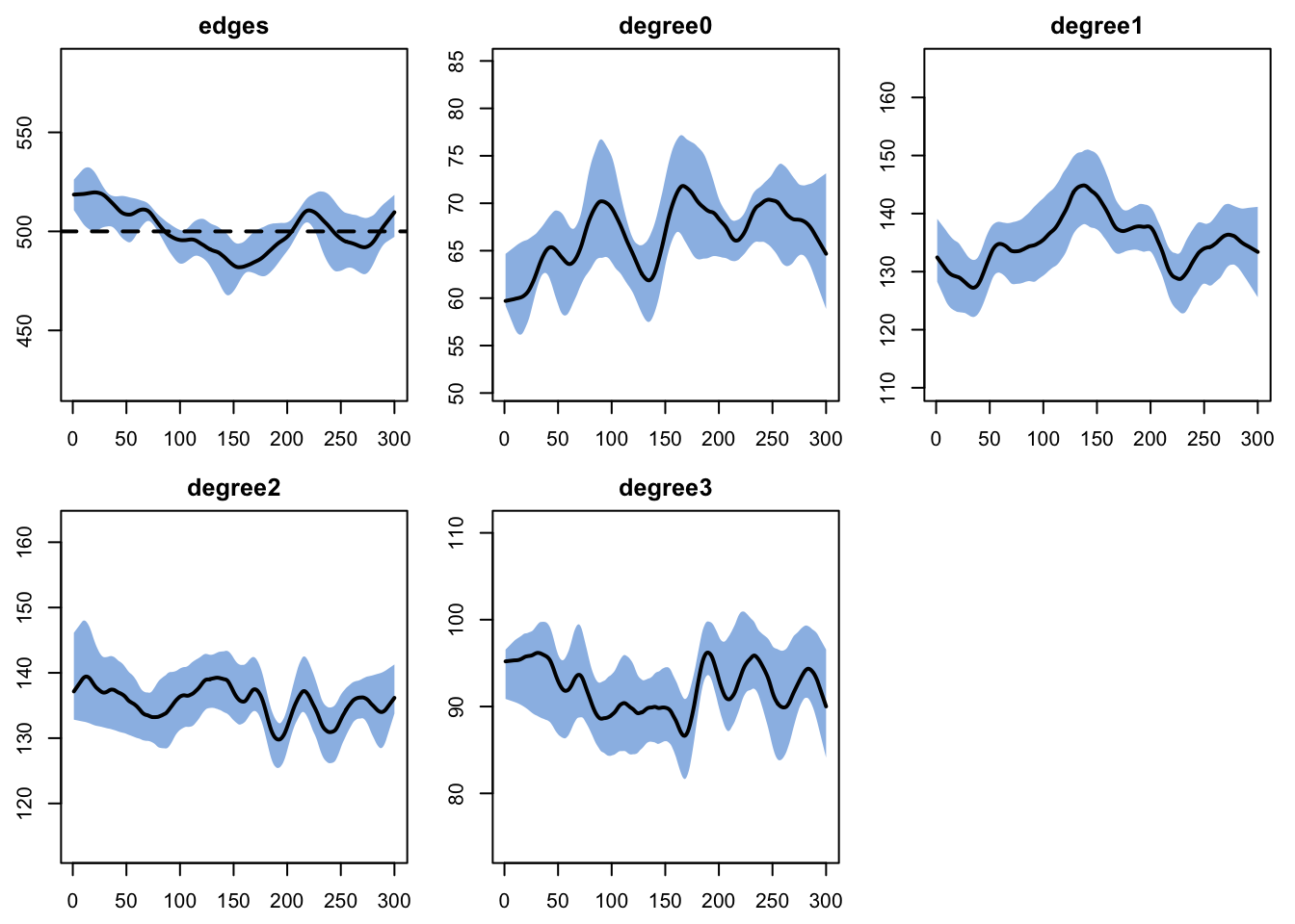
Parameters
Disease parameterization (each timestep treated as one day):
el.rate = 1/3: mean early sub-stage 3 days.lr.rate = 1/5: mean late sub-stage 5 days.- Total infectious period: 8 days.
Behavior multipliers applied to act.rate when the infected partner is in each sub-stage:
mult.early = 0.3(dynamic) or1.0(naive).mult.late = 0.6(dynamic) or1.0(naive).
make_param <- function(inf.prob,
                       mult.early = 1.0,
                       mult.late  = 1.0) {
  param.net(
    inf.prob   = inf.prob,
    act.rate   = 1,
    el.rate    = 1 / 3,
    lr.rate    = 1 / 5,
    mult.early = mult.early,
    mult.late  = mult.late
  )
}

init <- init.net(i.num = 10)

control <- control.net(
  type = NULL,
  nsims = nsims,
  ncores = ncores,
  nsteps = nsteps,
  infection.FUN = infect,
  progress.FUN  = progress,
  verbose = FALSE
)
Calibration
Both models are calibrated to the same cumulative attack rate (target 40%) by bisection on inf.prob. The relationship between inf.prob and the final attack rate is monotone on a closed population, so bisection converges reliably.
cum_attack <- function(sim) {
  df  <- as.data.frame(sim)
  inc <- tapply(df$si.flow, df$sim, sum, na.rm = TRUE)
  pop <- tapply(df$num,     df$sim, function(x) x[length(x)])
  mean(inc / pop, na.rm = TRUE)
}

calibrate_beta <- function(target, mult.early, mult.late,
                           lo = 0.01, hi = 0.60,
                           max_iter = cal_iter) {
  for (i in seq_len(max_iter)) {
    mid <- (lo + hi) / 2
    p   <- make_param(inf.prob   = mid,
                      mult.early = mult.early,
                      mult.late  = mult.late)
    sim <- netsim(est, p, init, control)
    ar  <- cum_attack(sim)
    if (is.na(ar) || ar < target) lo <- mid else hi <- mid
  }
  (lo + hi) / 2
}

target_attack <- 0.40
beta_dyn   <- calibrate_beta(target_attack, mult.early = 0.3, mult.late = 0.6)
beta_naive <- calibrate_beta(target_attack, mult.early = 1.0, mult.late = 1.0)

c(naive = beta_naive, dynamic = beta_dyn,
  ratio = beta_dyn / beta_naive)
naive dynamic ratio
0.1805469 0.3833594 2.1233232 The dynamic model needs a substantially higher inf.prob than the naive model to reproduce the same attack rate, because its infectious population spends part of the infectious period at reduced contact intensity. The ratio of calibrated values is approximately the inverse of the time-weighted mean of the early and late multipliers: (0.3 * 3 + 0.6 * 5) / 8 = 0.49, so the dynamic-to-naive ratio is approximately 1 / 0.49 ~ 2.05.
Calibrated Baseline Scenarios
sim_dyn   <- netsim(est,
                    make_param(beta_dyn,
                               mult.early = 0.3, mult.late = 0.6),
                    init, control)
sim_naive <- netsim(est,
                    make_param(beta_naive,
                               mult.early = 1.0, mult.late = 1.0),
                    init, control)
NPI Scenario: Isolation of Symptomatic Cases
The intervention drives mult.early down to a low absolute target (iso.mult = 0.1, which holds contact with every partner to 10% of the healthy rate during the most symptomatic phase). The late-stage multiplier is unchanged.
Same intervention, different starting points:
- Naive baseline
mult.earlywas 1.0, dropping to 0.1 is a 90% reduction in early-period contacts. - Dynamic baseline
mult.earlywas 0.3, dropping to 0.1 is a 67% reduction.
iso.mult <- 0.1

sim_dyn_npi   <- netsim(est,
                        make_param(beta_dyn,
                                   mult.early = iso.mult,
                                   mult.late  = 0.6),
                        init, control)
sim_naive_npi <- netsim(est,
                        make_param(beta_naive,
                                   mult.early = iso.mult,
                                   mult.late  = 1.0),
                        init, control)
Results
ar_dyn       <- cum_attack(sim_dyn)
ar_dyn_npi   <- cum_attack(sim_dyn_npi)
ar_naive     <- cum_attack(sim_naive)
ar_naive_npi <- cum_attack(sim_naive_npi)

red_dyn   <- 100 * (ar_dyn   - ar_dyn_npi)   / ar_dyn
red_naive <- 100 * (ar_naive - ar_naive_npi) / ar_naive

data.frame(
  Model       = c("Naive", "Dynamic"),
  inf.prob    = round(c(beta_naive,    beta_dyn),    4),
  Attack_base = round(c(ar_naive,      ar_dyn),      3),
  Attack_NPI  = round(c(ar_naive_npi,  ar_dyn_npi),  3),
  Pct_reduced = round(c(red_naive,     red_dyn),     1),
  row.names = NULL
)
Model inf.prob Attack_base Attack_NPI Pct_reduced
1 Naive 0.1805 0.312 0.112 64.3
2 Dynamic 0.3834 0.443 0.228 48.5Prevalence over time
Same calibration target, very different per-act transmissibility. The naive model needs a lower inf.prob because its infectious population is always at full contact intensity. The dynamic model needs a higher inf.prob to compensate for the reduced effective contacts during the symptomatic phase.
par(mfrow = c(1, 1), mar = c(3, 3, 2, 1), mgp = c(2, 1, 0))
plot(sim_naive, y = "i.num",
     main = "Calibrated Baseline Prevalence",
     ylab = "Number infectious",
     xlab = "Time step (days)",
     mean.col = "firebrick", mean.lwd = 2, mean.smooth = TRUE,
     qnts = FALSE, legend = FALSE,
     ylim = ylim_epi(list(sim_naive, sim_dyn), "i.num", qnts = FALSE))
plot(sim_dyn, y = "i.num",
     mean.col = "steelblue", mean.lwd = 2, mean.smooth = TRUE,
     qnts = FALSE, legend = FALSE, add = TRUE)
legend("topright",
       legend = c(sprintf("Naive (inf.prob=%.3f)",   beta_naive),
                  sprintf("Dynamic (inf.prob=%.3f)", beta_dyn)),
       col = c("firebrick", "steelblue"), lwd = 2, bty = "n")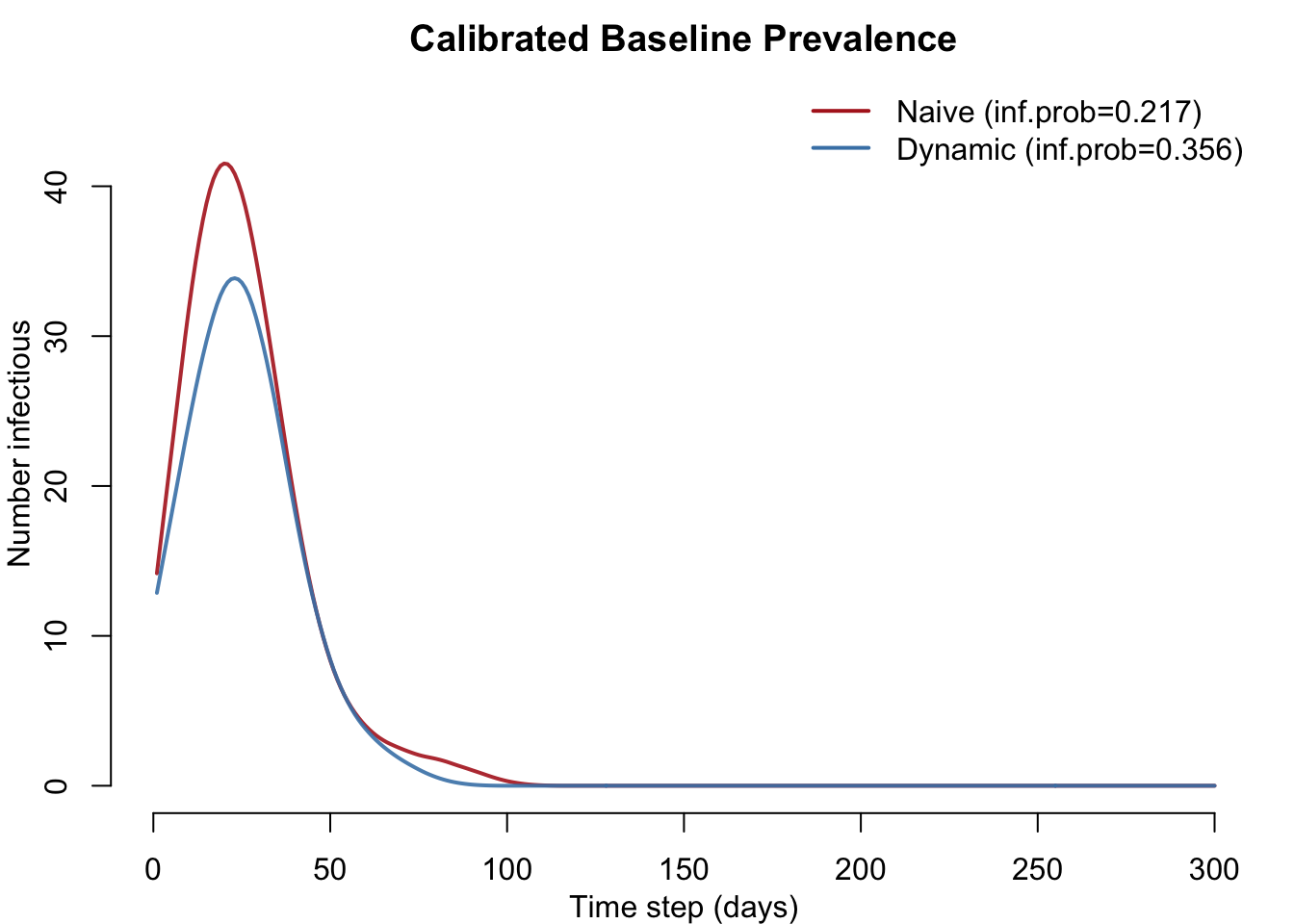
Calibrated transmissibility and NPI impact
The headline plot. Left: the naive model’s calibrated inf.prob is roughly half the dynamic model’s. Right: cumulative attack rate before and after the NPI for each model, with the signed percent change annotated under each pair (green = NPI lowered incidence, red = it did not). The dashed gray line marks the shared calibration target. The same intervention removes a larger share of incidence in the naive model than in the dynamic one.
par(mfrow = c(1, 2), mar = c(5, 4, 3, 1), mgp = c(2.4, 1, 0))

## Left: calibrated per-act transmission probability
bp1 <- barplot(c(Naive = beta_naive, Dynamic = beta_dyn),
               col = c("firebrick", "steelblue"),
               ylab = "Calibrated per-act transmission probability",
               main = "Calibrated Transmissibility",
               ylim = c(0, max(beta_naive, beta_dyn) * 1.25))
text(bp1, c(beta_naive, beta_dyn) * 1.07,
     sprintf("%.3f", c(beta_naive, beta_dyn)), font = 2)

## Right: baseline vs NPI attack rate, grouped by model
attack_mat <- matrix(c(ar_naive, ar_naive_npi,
                       ar_dyn,   ar_dyn_npi),
                     nrow = 2,
                     dimnames = list(c("Baseline", "NPI"),
                                     c("Naive", "Dynamic")))
cols_pair <- c(adjustcolor("firebrick", alpha.f = 0.45), "firebrick",
               adjustcolor("steelblue", alpha.f = 0.45), "steelblue")
ylim2 <- c(0, max(attack_mat, target_attack, na.rm = TRUE) * 1.3)

bp2 <- barplot(attack_mat, beside = TRUE,
               col = cols_pair, las = 1,
               ylab = "Cumulative attack rate",
               main = "Attack Rate: Baseline vs NPI",
               ylim = ylim2)

text(bp2, attack_mat + diff(ylim2) * 0.025,
     sprintf("%.2f", attack_mat), font = 2, cex = 0.9)

abline(h = target_attack, lty = 2, col = "gray40")

pct_change <- -c(red_naive, red_dyn)
mtext(side = 1, line = 2.4, at = colMeans(bp2),
      text = sprintf("%+.1f%%", pct_change),
      font = 2, cex = 0.95,
      col = ifelse(pct_change <= 0, "darkgreen", "firebrick"))

legend("topright",
       legend = c("Baseline", "+ NPI"),
       fill = c(adjustcolor("gray30", alpha.f = 0.45), "gray30"),
       border = NA, bty = "n", cex = 0.85)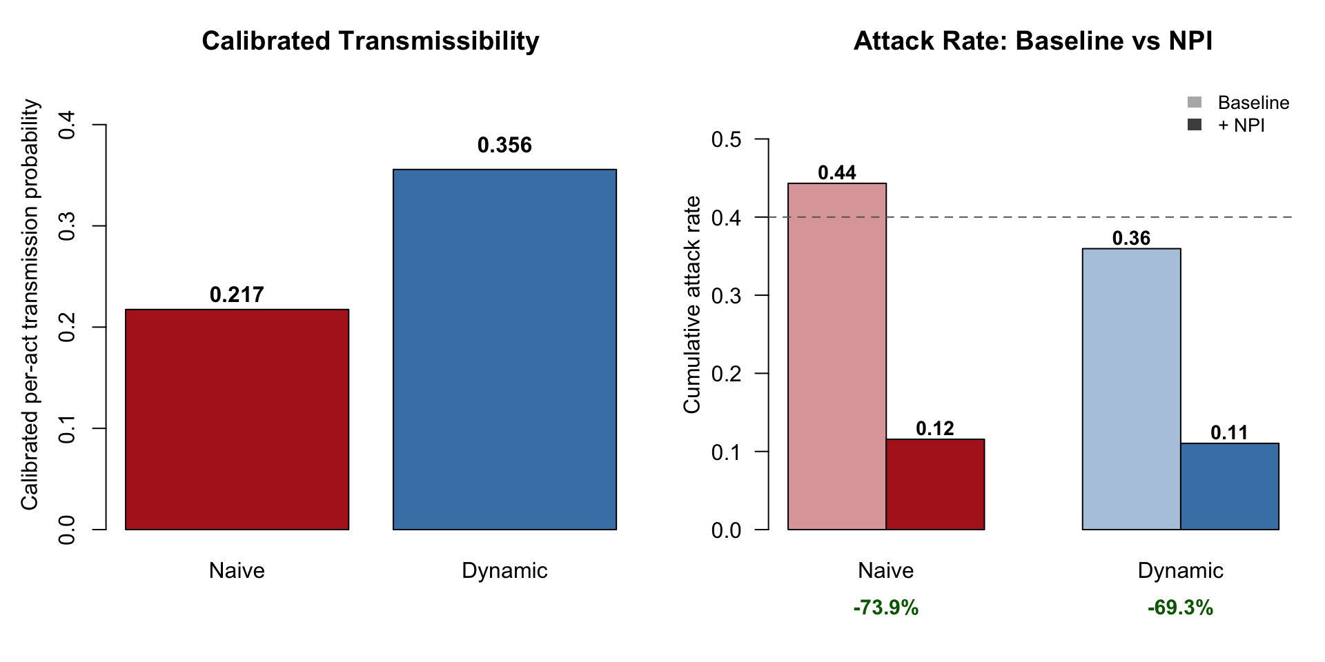
Interpretation
The two models are structurally identical and calibrated to the same observed attack rate. Their only difference is the assumption about contact behavior during the symptomatic period. Yet they project different intervention impacts: in this run the NPI reduces cumulative incidence by 64% in the naive model and by 48% in the dynamic model. The size of that gap is noisy at these settings, because each calibration step runs only 5 simulations of 500 people and the calibrated attack rates can land several points from the 40% target. Across six runs with different seeds, the naive projection was 1.3 to 2.2 times the dynamic one; it was the larger of the two in every run, and the naive model’s calibrated inf.prob was about half the dynamic model’s in every run.
The mechanism is straightforward. The naive model assumes sick people contact others at the same rate as healthy people. To match the observed attack rate under that assumption, the naive model must lower inf.prob. When the intervention then cuts contacts during the symptomatic period, the naive model removes a large slab of contact-time that the dynamic model never assigned to that period in the first place. The naive model gives itself more room to intervene than the dynamic model considers realistic.
The same logic applies to any model that assumes constant contact rates across an infectious period: when the underlying behavior is in fact stage-varying, calibrated transmissibility is biased downward and projected NPI impact is biased upward. The size of the bias scales with how much real behavior change is being ignored.
Next Steps
- Vary the multipliers to study sensitivity. Move
mult.earlyfrom 0.1 to 1.0 to span “perfect isolation” to “no behavior change” and watch the calibratedinf.proband NPI projections move together. - Add a pre-symptomatic stage that is infectious but contact-unchanged (relevant for some respiratory pathogens with substantial pre-symptomatic transmission).
- Layer on a population-level behavioral response: scale
mult.earlyandmult.lateby a function of current prevalence to model fear-driven contact reduction in addition to symptom-driven reduction.