Social Diffusion Model

social diffusion

complex contagion

intermediate

SI-based model comparing simple, threshold, and dose-response diffusion mechanisms on a social network

Author

Samuel M. Jenness

Published

September 1, 2018

Overview

This example demonstrates how EpiModel’s SI (susceptible-infected) framework can be repurposed to model social diffusion — the spread of ideas, behaviors, or technologies through a social network. Unlike infectious disease, social diffusion often exhibits complex contagion: adoption requires reinforcement from multiple contacts, not just exposure to a single carrier. The model compares three diffusion mechanisms on the same network to show how mechanism choice drives qualitatively different dynamics even when the network and initial conditions are identical.

The three mechanisms differ in what kind of hazard drives adoption:

Simple contagion (baseline). A per-edge per-contact hazard: each adopter-non-adopter edge independently fires at probability inf.prob per act. A non-adopter with more adopter contacts gets more independent chances — exposure has its effect through the number of contact events. This is EpiModel’s built-in SI module.
Threshold diffusion. A per-individual per-timestep hazard: each non-adopter draws once per timestep, with probability adopt.prob if their current exposure (number of adopter contacts) meets a minimum threshold, and probability zero otherwise.
Dose-response diffusion. Also a per-individual per-timestep hazard, with the probability rising smoothly with exposure via a logistic curve plogis(beta0 + beta1 * exposure). Like the threshold model, exposure of zero gives probability zero — diffusion requires exposure.

Both complex-contagion mechanisms are individual-level decision processes, in line with the social-contagion literature (Granovetter 1978; Watts 2002; Centola and Macy 2007). Exposure of zero gives an adoption probability of zero in both: a person cannot adopt a behavior they have never been exposed to through the network. Spontaneous adoption from outside the network is a separate “innovation” process and not part of these mechanisms.

The key insight is that the same well-connected network produces dramatically different diffusion trajectories depending on the mechanism. Simple contagion spreads fastest, following a classic S-curve. Threshold diffusion is dramatically delayed but then accelerates sharply once critical mass is reached. Dose-response diffusion falls between the two. Notably, the threshold model uses a per-individual adoption probability 5x higher than simple contagion’s per-contact probability, yet is still roughly 5x slower to reach 50% adoption — demonstrating that the mechanism of social influence matters more than the magnitude of the probability.

Download the Source Files

The complete source code for this example is available for download:

model.R: Main simulation script with all three diffusion scenarios
module-fx.R: Custom threshold and dose-response diffusion modules

Model Structure

This model uses SI (susceptible-infected) dynamics with no recovery, meaning adoption is permanent. The “S” compartment represents non-adopters and the “I” compartment represents adopters. The three scenarios differ only in how the adoption probability is calculated from a non-adopter’s exposure to adopter contacts.

Model compartments
Compartment	Label	Description
Non-Adopter	S	Has not yet adopted the behavior, idea, or technology
Adopter	I	Has adopted; can influence connected non-adopters

graph LR
    S["Non-Adopter (S)"] -->|"Adoption"| I["Adopter (I)"]

    style S fill:#4a90d9,stroke:#2c5f8a,color:#fff
    style I fill:#d94a4a,stroke:#8a2c2c,color:#fff

Diffusion flow diagram. Adoption is permanent (SI dynamics).

The critical distinction between the three scenarios is whether the hazard is per-edge (simple contagion) or per-individual (both complex-contagion mechanisms):

graph TD
    SIMPLE["<b>Simple Contagion</b><br/>Per-edge per-act<br/>P per act = inf.prob<br/>Draws: one per discordant edge"]
    EXP["Count adopter contacts<br/>per non-adopter (exposure)"]
    T["<b>Threshold</b><br/>P = adopt.prob if exposure >= min.degree<br/>P = 0 otherwise<br/>Draws: one per non-adopter"]
    D["<b>Dose-Response</b><br/>P = plogis(beta0 + beta1 * exposure) if exposure >= 1<br/>P = 0 if exposure = 0<br/>Draws: one per non-adopter"]

    EXP --> T
    EXP --> D

    style SIMPLE fill:#6aaa6a,stroke:#3d6b3d,color:#fff
    style EXP fill:#f5f5dc,stroke:#999
    style T fill:#d94a4a,stroke:#8a2c2c,color:#fff
    style D fill:#4a90d9,stroke:#2c5f8a,color:#fff

Adoption hazard by mechanism. Simple contagion fires Bernoulli draws on the discordant edgelist (per-edge per-act). Threshold and dose-response compute one adoption probability per non-adopter from their exposure count, then draw once.

Dose-Response Probability Curve

The logistic dose-response function with beta0 = -5.0 and beta1 = 1.5 produces these per-individual per-timestep adoption probabilities:

Dose-response adoption probabilities by exposure count
Adopter Contacts	Log-Odds	P(adopt per timestep)
0	–	0 (excluded)
1	-3.5	0.029
2	-2.0	0.119
3	-0.5	0.378
4	+1.0	0.731

By comparison, simple contagion uses a per-edge per-act probability of 0.1 (and a non-adopter with N adopter contacts effectively gets N independent draws). The threshold model uses a per-individual probability of 0.5 when exposure >= 2 and 0 otherwise.

Setup

We begin by loading EpiModel and setting the simulation parameters. The interactive() values are used here for richer output.

library(EpiModel)

nsims <- 5
ncores <- 5
nsteps <- 300

Custom Modules

The simple contagion scenario uses EpiModel’s built-in SI infection module, so no custom code is needed for that case. The two complex contagion scenarios each require a custom infection module that replaces the standard transmission logic with exposure-dependent adoption rules.

Threshold Diffusion Module

diffuse_threshold evaluates each non-adopter once per timestep. A non-adopter must have at least min.degree adopter contacts at this moment in time, or their adoption probability is exactly zero. Above that threshold, the probability is adopt.prob — a single Bernoulli draw per non-adopter, not one draw per adopter contact. This captures phenomena like technology adoption (“I’ll switch only if enough friends already use it”) or collective action (“I’ll join only if enough peers are committed”).

diffuse_threshold <- function(dat, at) {

  ## Attributes ##
  active <- get_attr(dat, "active")
  status <- get_attr(dat, "status")
  infTime <- get_attr(dat, "infTime")

  ## Parameters ##
  adopt.prob <- get_param(dat, "adopt.prob")
  min.degree <- get_param(dat, "min.degree")

  ## Candidate set: all active non-adopters ##
1  idsSus <- which(active == 1 & status == "s")
  nAdopt <- 0

  if (length(idsSus) > 0) {
2    # Per-individual exposure count (0 if no adopter contact)
    del <- discord_edgelist(dat, at)
    if (is.null(del) || nrow(del) == 0) {
      exposure_all <- integer(length(active))
    } else {
      exposure_all <- tabulate(del$sus, nbins = length(active))
    }
    sus_exposure <- exposure_all[idsSus]

3    # Per-individual adoption probability
    p <- ifelse(sus_exposure >= min.degree, adopt.prob, 0)

4    # Single Bernoulli draw per non-adopter per timestep
    idsNewAdopt <- idsSus[rbinom(length(idsSus), 1, p) == 1]
    nAdopt <- length(idsNewAdopt)

    if (nAdopt > 0) {
      status[idsNewAdopt] <- "i"
      infTime[idsNewAdopt] <- at
      dat <- set_attr(dat, "status", status)
      dat <- set_attr(dat, "infTime", infTime)
    }
  }

  ## Summary statistics ##
5  dat <- set_epi(dat, "si.flow", at, nAdopt)

  return(dat)
}

1: Candidate set is every non-adopter, not the discordant edgelist. This matters because a non-adopter with zero adopter contacts is still considered (and gets adoption probability zero), which makes the model match the literature’s per-individual decision framing.
2: tabulate(del$sus, nbins = N) returns a length-N vector counting how often each node appears as the susceptible end of a discordant edge. Non-adopters with no adopter contact get exposure 0 (not missing from the table).
3: Threshold rule applied at the individual level: adoption probability equals adopt.prob when current exposure meets the threshold, zero otherwise.
4: One Bernoulli draw per non-adopter, not one per edge. Exposure determines whether adoption is possible at all (via the threshold) and at what probability, but not how many independent chances per timestep.
5: The si.flow tracker records the number of new adoptions at each time step for later analysis.

Dose-Response Diffusion Module

diffuse_dose_response replaces the hard threshold with a smooth logistic curve: each non-adopter’s adoption probability rises gradually with their number of adopter contacts, plogis(beta0 + beta1 * exposure). Exposure of zero still gives probability zero (diffusion requires exposure); the smooth ramp simply removes the hard cutoff between “blocked” and “active” states. This is an intermediate model between simple contagion and threshold contagion.

diffuse_dose_response <- function(dat, at) {

  ## Attributes ##
  active <- get_attr(dat, "active")
  status <- get_attr(dat, "status")
  infTime <- get_attr(dat, "infTime")

  ## Parameters ##
  beta0 <- get_param(dat, "beta0")
  beta1 <- get_param(dat, "beta1")

  ## Candidate set: all active non-adopters ##
  idsSus <- which(active == 1 & status == "s")
  nAdopt <- 0

  if (length(idsSus) > 0) {
    del <- discord_edgelist(dat, at)
    if (is.null(del) || nrow(del) == 0) {
      exposure_all <- integer(length(active))
    } else {
      exposure_all <- tabulate(del$sus, nbins = length(active))
    }
    sus_exposure <- exposure_all[idsSus]

1    # Per-individual logistic dose-response.
    # Exposure-zero individuals are excluded: diffusion requires
    # at least one adopter contact.
    p <- ifelse(sus_exposure >= 1,
                plogis(beta0 + beta1 * sus_exposure),
                0)

2    idsNewAdopt <- idsSus[rbinom(length(idsSus), 1, p) == 1]
    nAdopt <- length(idsNewAdopt)

    if (nAdopt > 0) {
      status[idsNewAdopt] <- "i"
      infTime[idsNewAdopt] <- at
      dat <- set_attr(dat, "status", status)
      dat <- set_attr(dat, "infTime", infTime)
    }
  }

  ## Summary statistics ##
  dat <- set_epi(dat, "si.flow", at, nAdopt)

  return(dat)
}

1: Exposure-zero is structurally excluded. A non-adopter with no adopter contacts has adoption probability exactly zero, regardless of beta0. The logistic curve only governs the probability given at least one adopter contact, and beta0 sits at the bottom of the ramp (at exposure 1, plogis(beta0 + beta1)).
2: One Bernoulli draw per non-adopter per timestep, with probability determined by their current exposure. This is the individual-level decision framing from the social-contagion literature; it does not give a non-adopter additional independent chances simply because they have more adopter contacts (although those contacts do raise the per-decision probability via the logistic curve).

Network Model

Network Initialization

We initialize a 500-node network representing a social contact network. This could represent friendships, coworker relationships, or any social ties through which information or behavior can spread.

n <- 500
nw <- network_initialize(n)

Formation and Dissolution

The formation model targets 600 edges (mean degree = 2 x 600 / 500 = 2.4) with 20 isolated nodes (4% of the population). The isolates term controls how many nodes have degree 0, which shapes the degree distribution. A mean degree of 2.4 is important for the threshold model: with lower connectivity, requiring 2 adopter contacts would make diffusion nearly impossible because most nodes would not have enough contacts.

The partnership duration of 50 time steps represents stable social ties. Longer durations create a more stable network where people maintain the same connections over time, which is realistic for social relationships. This stability is important for the threshold model because non-adopters keep the same contacts for extended periods, meaning they must wait for those specific contacts to adopt (or for network turnover) before meeting the threshold requirement.

formation <- ~edges + isolates
target.stats <- c(600, 20)

coef.diss <- dissolution_coefs(dissolution = ~offset(edges), duration = 50)
coef.diss

Dissolution Coefficients
=======================
Dissolution Model: ~offset(edges)
Target Statistics: 50
Crude Coefficient: 3.89182
Mortality/Exit Rate: 0
Adjusted Coefficient: 3.89182

Network Estimation

est <- netest(nw, formation, target.stats, coef.diss)

Network Diagnostics

We verify that the simulated network maintains its target statistics and inspect the degree distribution. The degree distribution is particularly important here because complex contagion depends on having multiple adopter contacts, which requires sufficient connectivity (nodes with degree >= 2).

dx <- netdx(est, nsims = nsims, ncores = ncores, nsteps = nsteps,
            nwstats.formula = ~edges + isolates + degree(0:5))


Network Diagnostics
-----------------------
- Simulating 5 networks
- Calculating formation statistics

print(dx)

EpiModel Network Diagnostics
=======================
Diagnostic Method: Dynamic
Simulations: 5
Time Steps per Sim: 300

Formation Diagnostics
----------------------- 
         Target Sim Mean Pct Diff Sim SE Z Score SD(Sim Means) SD(Statistic)
edges       600  595.947   -0.675  2.770  -1.463         9.895        17.916
isolates     20   21.952    9.760  0.396   4.926         1.566         4.481
degree0      NA   21.952       NA  0.396      NA         1.566         4.481
degree1      NA  130.035       NA  1.076      NA         5.521        10.349
degree2      NA  142.731       NA  0.983      NA         3.693        10.136
degree3      NA  106.085       NA  0.897      NA         2.335         9.468
degree4      NA   57.501       NA  0.719      NA         0.990         7.301
degree5      NA   27.335       NA  0.426      NA         2.042         5.069

Duration Diagnostics
----------------------- 
      Target Sim Mean Pct Diff Sim SE Z Score SD(Sim Means) SD(Statistic)
edges     50   49.825    -0.35  0.352  -0.497         0.303         1.798

Dissolution Diagnostics
----------------------- 
      Target Sim Mean Pct Diff Sim SE Z Score SD(Sim Means) SD(Statistic)
edges   0.02     0.02     0.06      0    0.08             0         0.006

plot(dx)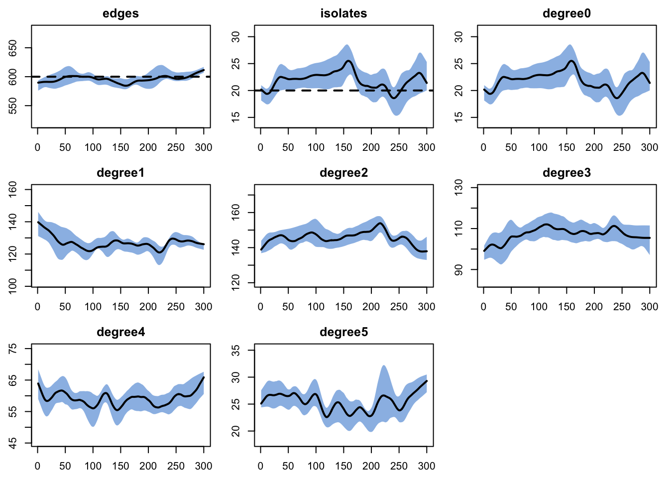

Figure 1: Network diagnostics showing target statistic tracking over time. The simulated network should maintain approximately 600 edges and 20 isolates throughout the simulation period.

Epidemic Simulation

All three scenarios share the same initial conditions: 50 initial adopters (10% seed prevalence). A meaningful seed is needed because the threshold model requires local clusters of adopters to form before diffusion can begin. With too few initial adopters on a stable network, the threshold model can stall entirely.

init <- init.net(i.num = 50)

Scenario 1: Simple Contagion (Baseline)

This scenario uses EpiModel’s built-in SI model. Each contact between an adopter and a non-adopter has a fixed probability of 0.1 of causing adoption, regardless of how many other adopter contacts the non-adopter has. This is the standard “simple contagion” assumption used in most epidemic models and serves as the reference case.

param_simple <- param.net(inf.prob = 0.1, act.rate = 1)

control_simple <- control.net(
  type = "SI",
  nsteps = nsteps,
  nsims = nsims,
  ncores = ncores,
  verbose = FALSE
)

sim_simple <- netsim(est, param_simple, init, control_simple)
print(sim_simple)

EpiModel Simulation
=======================
Model class: netsim

Simulation Summary
-----------------------
Model type: SI
No. simulations: 5
No. time steps: 300
No. NW groups: 1

Fixed Parameters
---------------------------
inf.prob = 0.1
act.rate = 1
groups = 1

Model Output
-----------------------
Variables: s.num i.num num si.flow
Networks: sim1 ... sim5
Transmissions: sim1 ... sim5

Formation Statistics
----------------------- 
         Target Sim Mean Pct Diff Sim SE Z Score SD(Sim Means) SD(Statistic)
edges       600  599.574   -0.071  3.135  -0.136         9.870        20.465
isolates     20   21.615    8.073  0.397   4.064         1.544         4.664


Duration Statistics
----------------------- 
      Target Sim Mean Pct Diff Sim SE Z Score SD(Sim Means) SD(Statistic)
edges     50   50.455     0.91  0.327    1.39         0.918         1.801

Dissolution Statistics
----------------------- 
      Target Sim Mean Pct Diff Sim SE Z Score SD(Sim Means) SD(Statistic)
edges   0.02     0.02   -1.294      0  -1.991             0         0.006

Scenario 2: Threshold Diffusion

A non-adopter only considers adoption when they have at least min.degree = 2 contacts who are already adopters. Below this threshold, the adoption probability is exactly zero. Once the threshold is met, each non-adopter draws once per timestep at adopt.prob = 0.5 — deliberately 5x higher than simple contagion’s 0.1 to demonstrate that the threshold mechanism still produces much slower diffusion despite the higher individual-level probability.

param_threshold <- param.net(adopt.prob = 0.5, min.degree = 2)

control_threshold <- control.net(
  type = NULL,
  nsteps = nsteps,
  nsims = nsims,
  ncores = ncores,
  infection.FUN = diffuse_threshold,
  verbose = FALSE
)

sim_threshold <- netsim(est, param_threshold, init, control_threshold)
print(sim_threshold)

EpiModel Simulation
=======================
Model class: netsim

Simulation Summary
-----------------------
Model type:
No. simulations: 5
No. time steps: 300
No. NW groups: 1

Fixed Parameters
---------------------------
adopt.prob = 0.5
min.degree = 2
act.rate = 1
groups = 1

Model Functions
-----------------------
initialize.FUN 
resim_nets.FUN 
summary_nets.FUN 
infection.FUN 
nwupdate.FUN 
prevalence.FUN 
verbose.FUN 

Model Output
-----------------------
Variables: s.num i.num num si.flow
Networks: sim1 ... sim5
Transmissions: sim1 ... sim5

Formation Statistics
----------------------- 
         Target Sim Mean Pct Diff Sim SE Z Score SD(Sim Means) SD(Statistic)
edges       600  591.634   -1.394  3.567  -2.345         5.129        19.578
isolates     20   21.792    8.960  0.449   3.992         0.586         4.937


Duration Statistics
----------------------- 
      Target Sim Mean Pct Diff Sim SE Z Score SD(Sim Means) SD(Statistic)
edges     50   49.639   -0.723  0.334  -1.083         1.227         1.889

Dissolution Statistics
----------------------- 
      Target Sim Mean Pct Diff Sim SE Z Score SD(Sim Means) SD(Statistic)
edges   0.02     0.02   -0.582      0  -0.823             0         0.006

Scenario 3: Dose-Response Diffusion

Adoption probability is a smooth logistic function of exposure: plogis(-5.0 + 1.5 * exposure) for exposure >= 1, and zero for exposure = 0. With a single adopter contact the probability is very low (0.029), so diffusion still requires meaningful social reinforcement. Unlike the threshold model, there is no hard cutoff between blocked and active states — the ramp from low to high adoption probability is smooth.

param_dose <- param.net(beta0 = -5.0, beta1 = 1.5)

control_dose <- control.net(
  type = NULL,
  nsteps = nsteps,
  nsims = nsims,
  ncores = ncores,
  infection.FUN = diffuse_dose_response,
  verbose = FALSE
)

sim_dose <- netsim(est, param_dose, init, control_dose)
print(sim_dose)

EpiModel Simulation
=======================
Model class: netsim

Simulation Summary
-----------------------
Model type:
No. simulations: 5
No. time steps: 300
No. NW groups: 1

Fixed Parameters
---------------------------
beta0 = -5
beta1 = 1.5
act.rate = 1
groups = 1

Model Functions
-----------------------
initialize.FUN 
resim_nets.FUN 
summary_nets.FUN 
infection.FUN 
nwupdate.FUN 
prevalence.FUN 
verbose.FUN 

Model Output
-----------------------
Variables: s.num i.num num si.flow
Networks: sim1 ... sim5
Transmissions: sim1 ... sim5

Formation Statistics
----------------------- 
         Target Sim Mean Pct Diff Sim SE Z Score SD(Sim Means) SD(Statistic)
edges       600  600.969    0.162  3.173   0.305         3.025        20.193
isolates     20   22.179   10.893  0.492   4.426         0.569         4.850


Duration Statistics
----------------------- 
      Target Sim Mean Pct Diff Sim SE Z Score SD(Sim Means) SD(Statistic)
edges     50    49.76    -0.48  0.348   -0.69         0.571         1.867

Dissolution Statistics
----------------------- 
      Target Sim Mean Pct Diff Sim SE Z Score SD(Sim Means) SD(Statistic)
edges   0.02     0.02   -0.607      0  -0.763             0         0.006

Analysis

Derived Measures

We compute adoption prevalence as a derived measure for all three scenarios to enable direct comparison.

sim_simple <- mutate_epi(sim_simple, prev = i.num / num)
sim_threshold <- mutate_epi(sim_threshold, prev = i.num / num)
sim_dose <- mutate_epi(sim_dose, prev = i.num / num)

Adoption Prevalence Comparison

This is the central comparison plot. All three scenarios use the same network and the same initial seed. The only difference is the mechanism by which exposure translates into adoption probability — simple is per-edge per-act, the two complex mechanisms are per-individual per-timestep.

par(mfrow = c(1, 1), mar = c(3, 3, 2, 1), mgp = c(2, 1, 0))

plot(sim_simple, y = "prev",
     main = "Adoption Prevalence: Three Diffusion Mechanisms",
     ylab = "Prevalence (Fraction Adopted)", xlab = "Time Steps",
     mean.col = "forestgreen", mean.lwd = 2, mean.smooth = TRUE,
     qnts.col = "forestgreen", qnts.alpha = 0.2, qnts.smooth = TRUE,
     legend = FALSE, ylim = c(0, 1))
plot(sim_threshold, y = "prev", add = TRUE,
     mean.col = "firebrick", mean.lwd = 2, mean.smooth = TRUE,
     qnts.col = "firebrick", qnts.alpha = 0.2, qnts.smooth = TRUE,
     legend = FALSE)
plot(sim_dose, y = "prev", add = TRUE,
     mean.col = "steelblue", mean.lwd = 2, mean.smooth = TRUE,
     qnts.col = "steelblue", qnts.alpha = 0.2, qnts.smooth = TRUE,
     legend = FALSE)
legend("bottomright",
       legend = c("Simple Contagion", "Threshold (min = 2)", "Dose-Response"),
       col = c("forestgreen", "firebrick", "steelblue"),
       lwd = 2, bty = "n")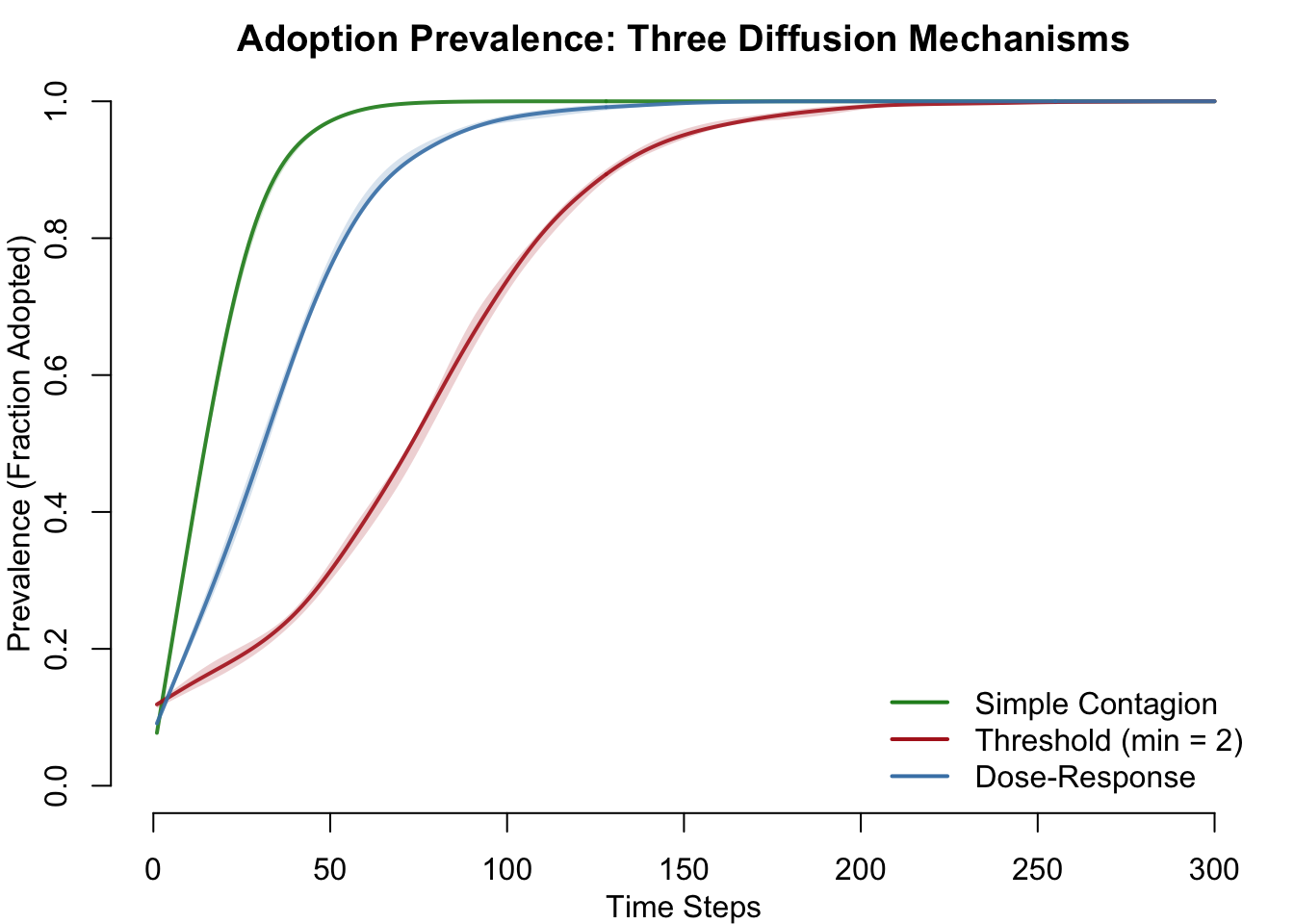

Figure 2: Adoption prevalence over time for the three diffusion mechanisms. Simple contagion (green) spreads fastest with a smooth S-curve. Threshold diffusion (red) shows delayed onset followed by rapid acceleration. Dose-response (blue) is intermediate. Shaded bands show interquartile ranges across simulations.

Adoption Incidence Comparison

The incidence plot shows the number of new adoptions per time step. Simple contagion produces a single smooth peak. Threshold diffusion shows a delayed, potentially sharper peak. Dose-response is intermediate.

par(mfrow = c(1, 1), mar = c(3, 3, 2, 1), mgp = c(2, 1, 0))

plot(sim_simple, y = "si.flow",
     main = "New Adoptions per Time Step",
     ylab = "New Adoptions", xlab = "Time Steps",
     mean.col = "forestgreen", mean.lwd = 2, mean.smooth = TRUE,
     qnts.col = "forestgreen", qnts.alpha = 0.2, qnts.smooth = TRUE,
     legend = FALSE)
plot(sim_threshold, y = "si.flow", add = TRUE,
     mean.col = "firebrick", mean.lwd = 2, mean.smooth = TRUE,
     qnts.col = "firebrick", qnts.alpha = 0.2, qnts.smooth = TRUE,
     legend = FALSE)
plot(sim_dose, y = "si.flow", add = TRUE,
     mean.col = "steelblue", mean.lwd = 2, mean.smooth = TRUE,
     qnts.col = "steelblue", qnts.alpha = 0.2, qnts.smooth = TRUE,
     legend = FALSE)
legend("topright",
       legend = c("Simple Contagion", "Threshold (min = 2)", "Dose-Response"),
       col = c("forestgreen", "firebrick", "steelblue"),
       lwd = 2, bty = "n")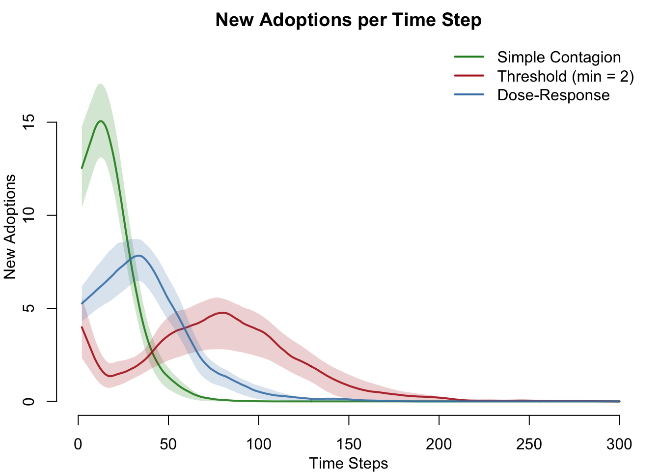

Figure 3: New adoptions per time step for each diffusion mechanism. The timing and shape of the incidence peak differs markedly across mechanisms, reflecting the different constraints on when adoption can occur.

Individual Scenario Detail

Each panel shows the non-adopter (S) and adopter (I) compartment counts for one scenario with quantile bands across simulations, revealing the stochastic variability within each mechanism.

par(mfrow = c(1, 3), mar = c(3, 3, 2, 1), mgp = c(2, 1, 0))

plot(sim_simple, y = c("s.num", "i.num"),
     main = "Simple Contagion",
     ylab = "Count", xlab = "Time Steps",
     mean.col = c("steelblue", "firebrick"),
     mean.lwd = 2, mean.smooth = TRUE,
     qnts.col = c("steelblue", "firebrick"),
     qnts.alpha = 0.2, qnts.smooth = TRUE,
     legend = TRUE)

plot(sim_threshold, y = c("s.num", "i.num"),
     main = "Threshold (min = 2)",
     ylab = "Count", xlab = "Time Steps",
     mean.col = c("steelblue", "firebrick"),
     mean.lwd = 2, mean.smooth = TRUE,
     qnts.col = c("steelblue", "firebrick"),
     qnts.alpha = 0.2, qnts.smooth = TRUE,
     legend = TRUE)

plot(sim_dose, y = c("s.num", "i.num"),
     main = "Dose-Response",
     ylab = "Count", xlab = "Time Steps",
     mean.col = c("steelblue", "firebrick"),
     mean.lwd = 2, mean.smooth = TRUE,
     qnts.col = c("steelblue", "firebrick"),
     qnts.alpha = 0.2, qnts.smooth = TRUE,
     legend = TRUE)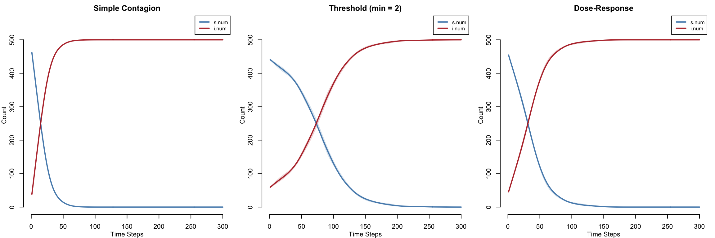

Figure 4: Compartment dynamics for each scenario. Left: simple contagion shows rapid, smooth transition. Center: threshold diffusion shows delayed onset and wider stochastic variability. Right: dose-response is intermediate.

Summary Table

df_simple <- as.data.frame(sim_simple)
df_threshold <- as.data.frame(sim_threshold)
df_dose <- as.data.frame(sim_dose)
last_t <- max(df_simple$time)

calc_t50 <- function(df) {
  mean_prev <- tapply(df$prev, df$time, mean, na.rm = TRUE)
  reached <- which(mean_prev >= 0.5)
  if (length(reached) == 0) NA else min(reached)
}
t50_simple <- calc_t50(df_simple)
t50_threshold <- calc_t50(df_threshold)
t50_dose <- calc_t50(df_dose)

summary_df <- data.frame(
  Metric = c("Final prevalence",
             "Time to 50% adoption",
             "Peak new adoptions/step",
             "Cumulative adoptions",
             "Mean prevalence"),
  Simple = c(round(mean(df_simple$prev[df_simple$time == last_t],
                        na.rm = TRUE), 3),
             t50_simple,
             round(max(tapply(df_simple$si.flow, df_simple$time,
                              mean, na.rm = TRUE), na.rm = TRUE), 1),
             round(sum(tapply(df_simple$si.flow, df_simple$time,
                              mean, na.rm = TRUE), na.rm = TRUE)),
             round(mean(df_simple$prev, na.rm = TRUE), 3)),
  Threshold = c(round(mean(df_threshold$prev[df_threshold$time == last_t],
                           na.rm = TRUE), 3),
                t50_threshold,
                round(max(tapply(df_threshold$si.flow, df_threshold$time,
                                 mean, na.rm = TRUE), na.rm = TRUE), 1),
                round(sum(tapply(df_threshold$si.flow, df_threshold$time,
                                 mean, na.rm = TRUE), na.rm = TRUE)),
                round(mean(df_threshold$prev, na.rm = TRUE), 3)),
  Dose_Response = c(round(mean(df_dose$prev[df_dose$time == last_t],
                               na.rm = TRUE), 3),
                    t50_dose,
                    round(max(tapply(df_dose$si.flow, df_dose$time,
                                     mean, na.rm = TRUE), na.rm = TRUE), 1),
                    round(sum(tapply(df_dose$si.flow, df_dose$time,
                                     mean, na.rm = TRUE), na.rm = TRUE)),
                    round(mean(df_dose$prev, na.rm = TRUE), 3))
)

knitr::kable(summary_df, col.names = c("Metric", "Simple", "Threshold", "Dose-Response"))

Table 1: Comparative summary statistics across the three diffusion mechanisms.

Metric	Simple	Threshold	Dose-Response
Final prevalence	1.000	1.000	1.000
Time to 50% adoption	15.000	90.000	33.000
Peak new adoptions/step	18.600	6.400	10.000
Cumulative adoptions	450.000	450.000	450.000
Mean prevalence	0.946	0.714	0.881

Parameters

Network Parameters

Network formation and dissolution parameters
Parameter	Value	Description
Network size	500	Total nodes in the social network
`edges` target	600	Mean degree = 2.4
`isolates` target	20	4% of nodes have no connections
Partnership duration	50	Average time steps per social tie

Scenario Parameters

Epidemic parameters by diffusion scenario
Parameter	Simple	Threshold	Dose-Response	Description
`inf.prob`	0.1	—	—	Per-edge per-act adoption probability (simple only)
`act.rate`	1	—	—	Acts per partnership per timestep (simple only)
`adopt.prob`	—	0.5	—	Per-individual per-timestep adoption probability when threshold met
`min.degree`	—	2	—	Minimum adopter contacts for adoption to be possible
`beta0`	—	—	-5.0	Logistic log-odds intercept
`beta1`	—	—	1.5	Logistic log-odds slope per adopter contact
Initial adopters	50	50	50	Seed prevalence = 10%

Simple contagion is parameterized as a per-edge per-act hazard (the disease-model convention). Threshold and dose-response use per-individual per-timestep hazards, which is why they have no act.rate.

Module Execution Order

All three scenarios follow the same module execution order at each time step. The only difference is the infection module used.

Module execution order at each time step
Order	Module	Function	Description
1	Resimulation	`resim_nets` (built-in)	Resimulate the dynamic network for the current time step
2	Infection	`infection.net` (simple) or `diffuse_threshold` or `diffuse_dose_response`	Compute adoption probability and determine new adopters
3	Prevalence	`prevalence.net` (built-in)	Update compartment counts and summary statistics

Next Steps

This example illustrates how EpiModel’s modular architecture allows the infection process to be completely replaced with custom diffusion logic. The same approach can be used to model other non-standard transmission processes. Related gallery examples include:

SEIR with Exposed State: Adds a latent period between exposure and infectiousness — a complementary way to model delayed onset dynamics.
SIS with Competing Strains: Models two competing behaviors or strains on the same network, which could be extended to competing innovations in a diffusion context.
SEIR with All-or-Nothing Vaccination: Demonstrates threshold-based protection mechanics that parallel the threshold diffusion concept.
Cost-Effectiveness Analysis: Shows how to attach outcome measures (costs, QALYs) to simulation results — applicable to evaluating diffusion intervention strategies.