Test and Treat Intervention for an SIS Epidemic

SIS

intervention

diagnosis

treatment

beginner

An SIS epidemic model with a test-and-treat intervention for a bacterial STI, comparing screening intensities on a dynamic sexual contact network.

Author

Samuel M. Jenness

Published

August 1, 2018

Overview

This example demonstrates how to build a test-and-treat intervention for a bacterial STI (e.g., gonorrhea) modeled as an SIS epidemic over a dynamic network. Many STIs are asymptomatic — infected individuals do not know they are infected without routine screening. Testing identifies infected individuals who then receive antibiotic treatment, dramatically accelerating recovery. The key question: how much screening is needed to meaningfully reduce population-level prevalence?

Unlike SIR models where recovered individuals gain immunity, the SIS framework allows reinfection — recovered individuals return to the susceptible pool and can be infected again. This creates an endemic equilibrium where new infections balance recoveries. Interventions that increase the recovery rate (like test-and-treat) shift this equilibrium to a lower prevalence.

This is the foundational intervention example in the Gallery. The techniques shown here — adding custom attributes for diagnosis status, implementing heterogeneous rates based on intervention status, and comparing intervention scenarios — are building blocks for more complex treatment cascade models.

Download standalone scripts

model.R — Main simulation script
module-fx.R — Custom module functions

Model Structure

Compartment	Label	Description
Susceptible	S	Not infected; at risk of infection (including previously recovered)
Infectious	I	Infected; can transmit to susceptible contacts

Within the infectious compartment, individuals can be either undiagnosed (recovering slowly via natural clearance) or diagnosed (recovering quickly via antibiotic treatment).

flowchart TD
    S["<b>S</b><br/>Susceptible"] -->|"infection<br/>(si.flow)"| I_undx

    subgraph Infected ["Infectious (I)"]
        I_undx["Undiagnosed<br/>rec.rate = 0.05"] -->|"testing<br/>(test.rate)"| I_dx["Diagnosed<br/>rec.rate.tx = 0.5"]
        I_dx -->|"test.dur expires"| I_undx
    end

    I_undx -->|"natural clearance<br/>(slow)"| S
    I_dx -->|"treatment<br/>(fast)"| S

    style S fill:#3498db,color:#fff
    style I_undx fill:#e74c3c,color:#fff
    style I_dx fill:#f39c12,color:#fff

In an SIS model, recovered individuals immediately return to the susceptible pool. There is no immune compartment, so the epidemic can persist indefinitely as an endemic equilibrium. Reinfection is common, and interventions must be sustained — unlike SIR vaccination, there is no herd immunity threshold.

The test-and-treat intervention follows a three-step cascade:

Testing: Undiagnosed individuals (both susceptible and infected) test at rate test.rate per timestep. Testing is universal — it does not require symptoms.
Diagnosis: Tested individuals receive diag.status = 1. For infected individuals, this triggers faster recovery at rate rec.rate.tx.
Treatment course: Diagnosis persists for test.dur timesteps. If the individual has not recovered by then, their diagnosis resets and they return to the natural clearance rate until re-tested.

On recovery, diagnosis status is always cleared (the individual is cured and no longer in the treatment pipeline).

Setup

suppressMessages(library(EpiModel))

nsims <- 5
ncores <- 5
nsteps <- 500

Custom Modules

Test and Treat Module

This module implements the screening and diagnosis cascade. At each timestep, undiagnosed individuals test with probability test.rate. Newly tested individuals receive a diagnosis that persists for test.dur timesteps, after which it resets. Both susceptible and infected individuals are eligible for testing — the key is that diagnosed infected individuals recover at the faster treatment rate in the recovery module.

tnt <- function(dat, at) {

  ## Attributes ##
  active <- get_attr(dat, "active")

1  if (at == 2) {
    dat <- set_attr(dat, "diag.status", rep(0, length(active)))
    dat <- set_attr(dat, "diag.time", rep(NA, length(active)))
  }
  diag.status <- get_attr(dat, "diag.status")
  diag.time <- get_attr(dat, "diag.time")

  ## Parameters ##
  test.rate <- get_param(dat, "test.rate")
  test.dur <- get_param(dat, "test.dur")

  ## Testing process ##
2  idsElig <- which(active == 1 & diag.status == 0)
  nElig <- length(idsElig)

3  vecTest <- which(rbinom(nElig, 1, test.rate) == 1)
  idsTest <- idsElig[vecTest]
  nTest <- length(idsTest)

  ## Update diagnosis status for newly tested ##
  diag.status[idsTest] <- 1
  diag.time[idsTest] <- at

  ## Diagnosis reset ##
4  idsReset <- which(at - diag.time > (test.dur - 1))
  diag.status[idsReset] <- 0
  diag.time[idsReset] <- NA

  ## Write out updated attributes ##
  dat <- set_attr(dat, "diag.status", diag.status)
  dat <- set_attr(dat, "diag.time", diag.time)

  ## Summary statistics ##
  dat <- set_epi(dat, "nTest", at, nTest)
  dat <- set_epi(dat, "nRest", at, length(idsReset))
  dat <- set_epi(dat, "nDiag", at, sum(diag.status == 1, na.rm = TRUE))

  return(dat)
}

1: Custom attributes (diag.status, diag.time) are initialized at timestep 2 because timestep 1 is reserved for init.net setup.
2: All active, undiagnosed individuals are eligible for testing — both susceptible and infected. Testing does not require symptoms.
3: Each eligible individual independently tests with probability test.rate per timestep (Bernoulli trial).
4: Diagnosis resets after test.dur timesteps. If the individual is still infected, they return to the slower natural clearance rate until re-tested.

Recovery Module

This module replaces EpiModel’s built-in recovery module to implement heterogeneous recovery rates. Diagnosed individuals recover at rec.rate.tx (fast, antibiotic treatment) while undiagnosed individuals recover at rec.rate (slow, natural clearance). This is the core mechanism of the test-and-treat intervention: screening accelerates recovery for those diagnosed, reducing their infectious duration and thereby suppressing transmission.

recov <- function(dat, at) {

  ## Attributes ##
  active <- get_attr(dat, "active")
  status <- get_attr(dat, "status")
  diag.status <- get_attr(dat, "diag.status")

  ## Parameters ##
  rec.rate <- get_param(dat, "rec.rate")
  rec.rate.tx <- get_param(dat, "rec.rate.tx")

  ## Determine eligible to recover ##
  idsElig <- which(active == 1 & status == "i")
  nElig <- length(idsElig)

  ## Heterogeneous recovery rates based on diagnosis status ##
  diag.status.elig <- diag.status[idsElig]
1  ratesElig <- ifelse(diag.status.elig == 1, rec.rate.tx, rec.rate)

  ## Stochastic recovery process ##
2  vecRecov <- which(rbinom(nElig, 1, ratesElig) == 1)
  idsRecov <- idsElig[vecRecov]
  nRecov <- length(idsRecov)

  ## Update attributes for recovered individuals ##
3  status[idsRecov] <- "s"
  diag.status[idsRecov] <- 0

  ## Write out updated attributes ##
  dat <- set_attr(dat, "status", status)
  dat <- set_attr(dat, "diag.status", diag.status)

  ## Summary statistics ##
  dat <- set_epi(dat, "is.flow", at, nRecov)

  return(dat)
}

1: The core intervention mechanism: diagnosed individuals recover at rec.rate.tx (0.5, mean ~2 weeks) while undiagnosed recover at rec.rate (0.05, mean ~20 weeks) — a 10x difference.
2: Each infected individual independently recovers with their diagnosis-specific probability (Bernoulli trial with heterogeneous rates).
3: Recovery clears both disease status (back to susceptible) and diagnosis status, since the individual is cured and exits the treatment pipeline.

Network Model

The formation model uses three ERGM terms to create a realistic sexual contact network for STI transmission.

n <- 500
nw <- network_initialize(n)

1formation <- ~edges + concurrent + degrange(from = 4)
2target.stats <- c(175, 110, 0)

3coef.diss <- dissolution_coefs(dissolution = ~offset(edges), duration = 50)
coef.diss

est <- netest(nw, formation, target.stats, coef.diss)

1: Three ERGM terms: edges controls mean degree, concurrent controls overlapping partnerships (degree > 1), and degrange(from = 4) prevents unrealistically high-degree nodes.
2: Targets: 175 edges (mean degree 0.7), 110 concurrent nodes (22% of the population), and zero nodes with 4+ simultaneous partners.
3: Mean partnership duration of 50 weeks (~1 year).

Dissolution Coefficients
=======================
Dissolution Model: ~offset(edges)
Target Statistics: 50
Crude Coefficient: 3.89182
Mortality/Exit Rate: 0
Adjusted Coefficient: 3.89182

Network Diagnostics

dx <- netdx(est, nsims = nsims, ncores = ncores, nsteps = nsteps,
            nwstats.formula = ~edges + concurrent + degree(0:5))


Network Diagnostics
-----------------------
- Simulating 5 networks
- Calculating formation statistics

print(dx)

EpiModel Network Diagnostics
=======================
Diagnostic Method: Dynamic
Simulations: 5
Time Steps per Sim: 500

Formation Diagnostics
----------------------- 
           Target Sim Mean Pct Diff Sim SE Z Score SD(Sim Means) SD(Statistic)
edges         175  180.299    3.028  1.878   2.822         2.145        11.656
concurrent    110  113.423    3.112  1.334   2.565         2.685        11.134
degree0        NA  266.827       NA  2.437      NA         1.648        12.941
degree1        NA  119.750       NA  1.003      NA         2.203         9.818
degree2        NA   99.421       NA  1.205      NA         2.290        10.442
degree3        NA   14.002       NA  0.392      NA         0.907         3.785
degree4        NA    0.000       NA    NaN      NA         0.000         0.000
degree5        NA    0.000       NA    NaN      NA         0.000         0.000

Duration Diagnostics
----------------------- 
      Target Sim Mean Pct Diff Sim SE Z Score SD(Sim Means) SD(Statistic)
edges     50    50.87    1.739  0.637   1.366         1.933         3.901

Dissolution Diagnostics
----------------------- 
      Target Sim Mean Pct Diff Sim SE Z Score SD(Sim Means) SD(Statistic)
edges   0.02     0.02   -2.271      0  -2.238         0.001         0.011

plot(dx)

Figure 1: Network diagnostic plots verifying the simulation reproduces the target statistics for edges, concurrency, and degree distribution.

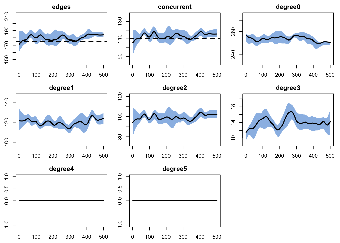
Epidemic Simulation

Initial Conditions and Control Settings

All three scenarios share the same initial conditions and control settings. The control.net call registers the built-in infection module alongside the two custom modules (test-and-treat and recovery).

1init <- init.net(i.num = 10)

control <- control.net(
2  type = NULL,
  nsims = nsims,
  ncores = ncores,
  nsteps = nsteps,
3  infection.FUN = infection.net,
  recovery.FUN = recov,
  tnt.FUN = tnt,
  verbose = FALSE
)

1: Seed the epidemic with 10 infected nodes (2% of the 500-node population).
2: type = NULL tells EpiModel that all modules are explicitly specified — no built-in SIS/SIR logic.
3: infection.net is EpiModel’s built-in SI infection module; recov and tnt are the custom modules defined above.

Scenario 1: No Screening (SIS Baseline)

Without any screening, only natural clearance (rec.rate = 0.05) drives recovery. The SIS model reaches an endemic equilibrium where new infections balance natural recoveries. This is the counterfactual — what happens without intervention.

param_none <- param.net(
  inf.prob = 0.4, act.rate = 2,
  rec.rate = 1 / 20, rec.rate.tx = 0.5,
  test.rate = 0, test.dur = 2
)

sim_none <- netsim(est, param_none, init, control)
print(sim_none)

EpiModel Simulation
=======================
Model class: netsim

Simulation Summary
-----------------------
Model type:
No. simulations: 5
No. time steps: 500
No. NW groups: 1

Fixed Parameters
---------------------------
inf.prob = 0.4
act.rate = 2
rec.rate = 0.05
rec.rate.tx = 0.5
test.rate = 0
test.dur = 2
groups = 1

Model Functions
-----------------------
initialize.FUN 
resim_nets.FUN 
summary_nets.FUN 
infection.FUN 
recovery.FUN 
nwupdate.FUN 
prevalence.FUN 
verbose.FUN 
tnt.FUN 

Model Output
-----------------------
Variables: s.num i.num num nTest nRest nDiag si.flow 
is.flow
Networks: sim1 ... sim5
Transmissions: sim1 ... sim5

Formation Statistics
----------------------- 
           Target Sim Mean Pct Diff Sim SE Z Score SD(Sim Means) SD(Statistic)
edges         175  178.379    1.931  2.787   1.213         8.253        15.882
concurrent    110  111.552    1.411  1.741   0.891         6.633        13.936
deg4+           0    0.000      NaN    NaN     NaN         0.000         0.000


Duration Statistics
----------------------- 
      Target Sim Mean Pct Diff Sim SE Z Score SD(Sim Means) SD(Statistic)
edges     50   50.072    0.144  0.467   0.154         0.959         3.302

Dissolution Statistics
----------------------- 
      Target Sim Mean Pct Diff Sim SE Z Score SD(Sim Means) SD(Statistic)
edges   0.02     0.02   -0.897      0  -0.871         0.001          0.01

Scenario 2: Standard Screening

10% of undiagnosed individuals test each week (~10-week average interval between tests). This represents a moderate screening program — feasible for clinical settings with annual or semi-annual testing recommendations.

param_std <- param.net(
  inf.prob = 0.4, act.rate = 2,
  rec.rate = 1 / 20, rec.rate.tx = 0.5,
  test.rate = 0.1, test.dur = 2
)

sim_std <- netsim(est, param_std, init, control)
print(sim_std)

EpiModel Simulation
=======================
Model class: netsim

Simulation Summary
-----------------------
Model type:
No. simulations: 5
No. time steps: 500
No. NW groups: 1

Fixed Parameters
---------------------------
inf.prob = 0.4
act.rate = 2
rec.rate = 0.05
rec.rate.tx = 0.5
test.rate = 0.1
test.dur = 2
groups = 1

Model Functions
-----------------------
initialize.FUN 
resim_nets.FUN 
summary_nets.FUN 
infection.FUN 
recovery.FUN 
nwupdate.FUN 
prevalence.FUN 
verbose.FUN 
tnt.FUN 

Model Output
-----------------------
Variables: s.num i.num num nTest nRest nDiag si.flow 
is.flow
Networks: sim1 ... sim5
Transmissions: sim1 ... sim5

Formation Statistics
----------------------- 
           Target Sim Mean Pct Diff Sim SE Z Score SD(Sim Means) SD(Statistic)
edges         175  174.482   -0.296  2.963  -0.175         5.698        15.501
concurrent    110  109.330   -0.609  1.825  -0.367         4.569        13.267
deg4+           0    0.000      NaN    NaN     NaN         0.000         0.000


Duration Statistics
----------------------- 
      Target Sim Mean Pct Diff Sim SE Z Score SD(Sim Means) SD(Statistic)
edges     50   49.278   -1.443  0.495  -1.458         1.273         3.269

Dissolution Statistics
----------------------- 
      Target Sim Mean Pct Diff Sim SE Z Score SD(Sim Means) SD(Statistic)
edges   0.02     0.02    1.683      0   1.546             0         0.011

Scenario 3: Intensive Screening

30% of undiagnosed individuals test each week (~3-week average interval). This represents an aggressive public health intervention — frequent screening in high-prevalence populations.

param_int <- param.net(
  inf.prob = 0.4, act.rate = 2,
  rec.rate = 1 / 20, rec.rate.tx = 0.5,
  test.rate = 0.3, test.dur = 2
)

sim_int <- netsim(est, param_int, init, control)
print(sim_int)

EpiModel Simulation
=======================
Model class: netsim

Simulation Summary
-----------------------
Model type:
No. simulations: 5
No. time steps: 500
No. NW groups: 1

Fixed Parameters
---------------------------
inf.prob = 0.4
act.rate = 2
rec.rate = 0.05
rec.rate.tx = 0.5
test.rate = 0.3
test.dur = 2
groups = 1

Model Functions
-----------------------
initialize.FUN 
resim_nets.FUN 
summary_nets.FUN 
infection.FUN 
recovery.FUN 
nwupdate.FUN 
prevalence.FUN 
verbose.FUN 
tnt.FUN 

Model Output
-----------------------
Variables: s.num i.num num nTest nRest nDiag si.flow 
is.flow
Networks: sim1 ... sim5
Transmissions: sim1 ... sim5

Formation Statistics
----------------------- 
           Target Sim Mean Pct Diff Sim SE Z Score SD(Sim Means) SD(Statistic)
edges         175  177.040    1.166  1.914   1.066         5.050        11.990
concurrent    110  110.774    0.703  1.297   0.597         4.043        10.741
deg4+           0    0.000      NaN    NaN     NaN         0.000         0.000


Duration Statistics
----------------------- 
      Target Sim Mean Pct Diff Sim SE Z Score SD(Sim Means) SD(Statistic)
edges     50   49.712   -0.576  0.675  -0.426         1.158         3.871

Dissolution Statistics
----------------------- 
      Target Sim Mean Pct Diff Sim SE Z Score SD(Sim Means) SD(Statistic)
edges   0.02     0.02    1.086      0   1.071             0         0.011

Analysis

sim_none <- mutate_epi(sim_none, prev = i.num / num)
sim_std <- mutate_epi(sim_std, prev = i.num / num)
sim_int <- mutate_epi(sim_int, prev = i.num / num)

Prevalence Comparison

The central question: how does screening intensity affect population-level STI prevalence? Without screening, the model reaches an endemic equilibrium at roughly 45%. Standard screening reduces prevalence to approximately 30%, and intensive screening pushes it to near elimination.

par(mfrow = c(1, 1), mar = c(3, 3, 2, 1), mgp = c(2, 1, 0))
plot(sim_none, y = "prev",
     main = "Prevalence by Screening Intensity",
     ylab = "Prevalence (I / N)", xlab = "Week",
     mean.col = "firebrick", mean.lwd = 2, mean.smooth = TRUE,
     qnts.col = "firebrick", qnts.alpha = 0.2, qnts.smooth = TRUE,
     legend = FALSE)
plot(sim_std, y = "prev",
     mean.col = "steelblue", mean.lwd = 2, mean.smooth = TRUE,
     qnts.col = "steelblue", qnts.alpha = 0.2, qnts.smooth = TRUE,
     legend = FALSE, add = TRUE)
plot(sim_int, y = "prev",
     mean.col = "seagreen", mean.lwd = 2, mean.smooth = TRUE,
     qnts.col = "seagreen", qnts.alpha = 0.2, qnts.smooth = TRUE,
     legend = FALSE, add = TRUE)
legend("topright",
       legend = c("No Screening", "Standard (10%/wk)", "Intensive (30%/wk)"),
       col = c("firebrick", "steelblue", "seagreen"), lwd = 2, bty = "n")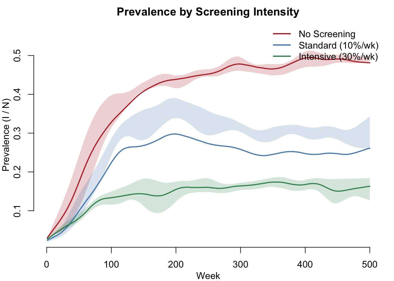

Figure 2: Prevalence over time under three screening intensities. Red: no screening (endemic equilibrium). Blue: standard screening (10%/week). Green: intensive screening (30%/week).

Compartment Dynamics

A side-by-side comparison of susceptible and infectious compartment counts. Without screening, the SIS model reaches a stable endemic equilibrium with a large infected pool. Intensive screening suppresses the infectious compartment dramatically.

par(mfrow = c(1, 2), mar = c(3, 3, 2, 1), mgp = c(2, 1, 0))
plot(sim_none, y = c("s.num", "i.num"),
     main = "No Screening",
     mean.col = c("steelblue", "firebrick"), mean.lwd = 2, mean.smooth = TRUE,
     qnts = FALSE, legend = TRUE)
plot(sim_int, y = c("s.num", "i.num"),
     main = "Intensive Screening",
     mean.col = c("steelblue", "firebrick"), mean.lwd = 2, mean.smooth = TRUE,
     qnts = FALSE, legend = TRUE)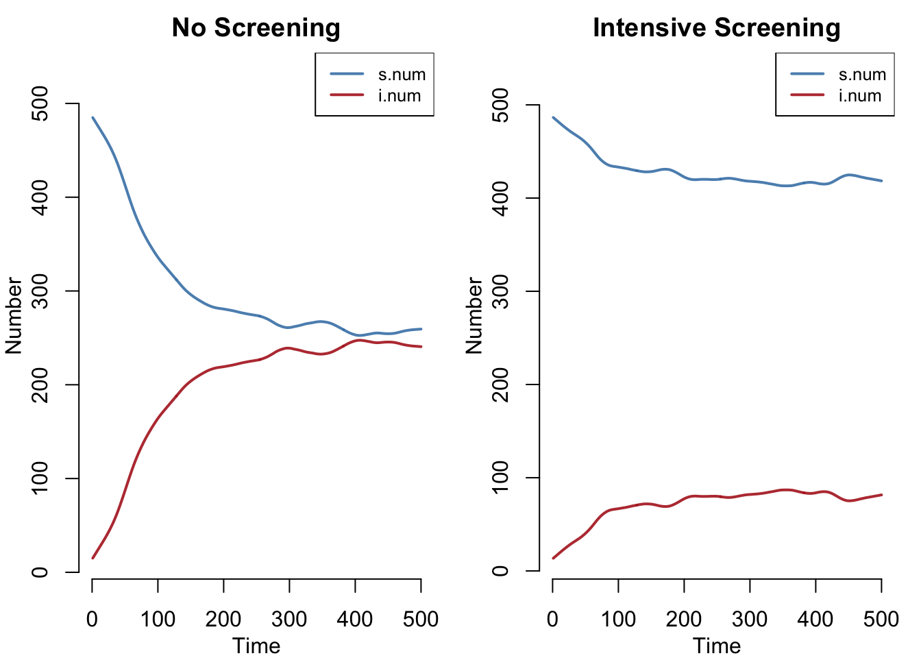

Figure 3: Compartment dynamics (S and I counts) under no screening (left) and intensive screening (right).

Diagnosis Coverage

How many individuals are currently diagnosed at each timestep? This shows the test-and-treat cascade in action — the fraction of infected individuals who are in the treatment pipeline.

par(mfrow = c(1, 1), mar = c(3, 3, 2, 1), mgp = c(2, 1, 0))
plot(sim_std, y = "nDiag",
     main = "Currently Diagnosed (Treatment Pipeline)",
     ylab = "Number Diagnosed", xlab = "Week",
     mean.col = "steelblue", mean.lwd = 2, mean.smooth = TRUE,
     qnts.col = "steelblue", qnts.alpha = 0.2, qnts.smooth = TRUE,
     legend = FALSE)
plot(sim_int, y = "nDiag",
     mean.col = "#27ae60", mean.lwd = 2, mean.smooth = TRUE,
     qnts.col = "#27ae60", qnts.alpha = 0.2, qnts.smooth = TRUE,
     legend = FALSE, add = TRUE)
legend("topright",
       legend = c("Standard (10%/wk)", "Intensive (30%/wk)"),
       col = c("steelblue", "#27ae60"), lwd = 2, bty = "n")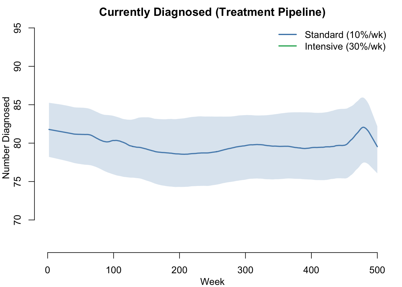

Figure 4: Number of currently diagnosed individuals over time for the standard and intensive screening scenarios.

Incidence

Incidence (new infections per week) shows the epidemic’s momentum. Without screening, incidence stabilizes at a high endemic level. With screening, incidence drops as fewer infected individuals are available to transmit.

par(mfrow = c(1, 1), mar = c(3, 3, 2, 1), mgp = c(2, 1, 0))
plot(sim_none, y = "si.flow",
     main = "New Infections per Week",
     ylab = "New Infections", xlab = "Week",
     mean.col = "firebrick", mean.lwd = 2, mean.smooth = TRUE,
     qnts.col = "firebrick", qnts.alpha = 0.2, qnts.smooth = TRUE,
     legend = FALSE)
plot(sim_std, y = "si.flow",
     mean.col = "steelblue", mean.lwd = 2, mean.smooth = TRUE,
     qnts.col = "steelblue", qnts.alpha = 0.2, qnts.smooth = TRUE,
     legend = FALSE, add = TRUE)
plot(sim_int, y = "si.flow",
     mean.col = "#27ae60", mean.lwd = 2, mean.smooth = TRUE,
     qnts.col = "#27ae60", qnts.alpha = 0.2, qnts.smooth = TRUE,
     legend = FALSE, add = TRUE)
legend("topright",
       legend = c("No Screening", "Standard (10%/wk)", "Intensive (30%/wk)"),
       col = c("firebrick", "steelblue", "#27ae60"), lwd = 2, bty = "n")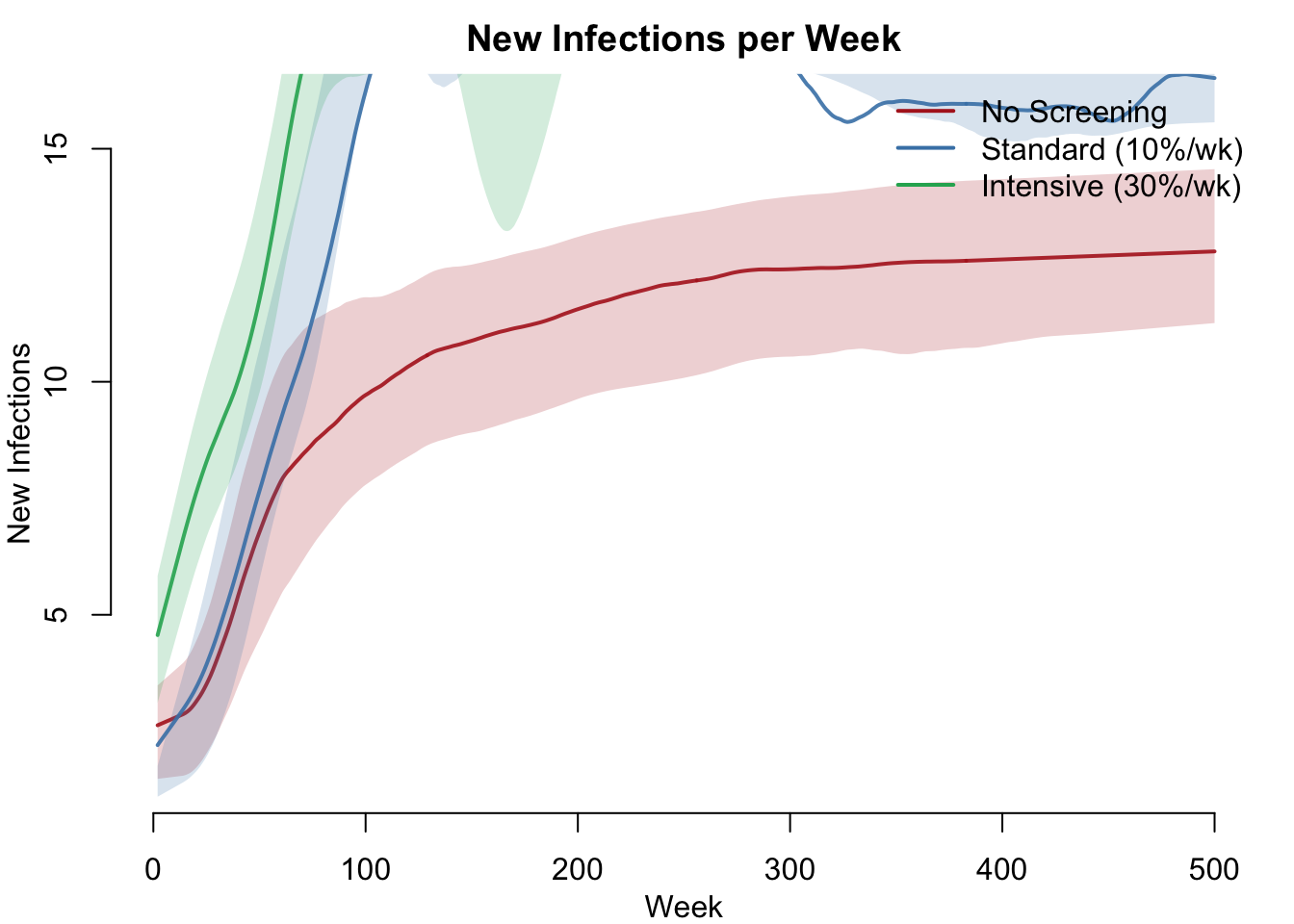

Figure 5: Weekly new infections across the three screening scenarios.

Summary Table

In an SIS model, the right burden metric is person-weeks infected (total time spent in the I compartment across all individuals), not cumulative new infections. Cumulative infections can paradoxically increase with screening because treated individuals recover faster, become susceptible again, and get reinfected.

df_none <- as.data.frame(sim_none)
df_std <- as.data.frame(sim_std)
df_int <- as.data.frame(sim_int)

pw_none <- mean(tapply(df_none$i.num, df_none$sim, sum, na.rm = TRUE))
pw_std <- mean(tapply(df_std$i.num, df_std$sim, sum, na.rm = TRUE))
pw_int <- mean(tapply(df_int$i.num, df_int$sim, sum, na.rm = TRUE))

knitr::kable(data.frame(
  Metric = c("Equilibrium prevalence",
             "Person-weeks infected",
             "Burden reduction (vs. none)",
             "Mean diagnosed (nDiag)"),
  No_Screening = c(
    round(mean(df_none$prev[df_none$time > nsteps * 0.8], na.rm = TRUE), 3),
    round(pw_none),
    "---",
    0
  ),
  Standard = c(
    round(mean(df_std$prev[df_std$time > nsteps * 0.8], na.rm = TRUE), 3),
    round(pw_std),
    paste0(round((1 - pw_std / pw_none) * 100), "%"),
    round(mean(df_std$nDiag[df_std$time > nsteps * 0.8], na.rm = TRUE), 1)
  ),
  Intensive = c(
    round(mean(df_int$prev[df_int$time > nsteps * 0.8], na.rm = TRUE), 3),
    round(pw_int),
    paste0(round((1 - pw_int / pw_none) * 100), "%"),
    round(mean(df_int$nDiag[df_int$time > nsteps * 0.8], na.rm = TRUE), 1)
  )
))

Table 1

Metric	No_Screening	Standard	Intensive
Equilibrium prevalence	0.489	0.248	0.16
Person-weeks infected	99912	57553	35771
Burden reduction (vs. none)	—	42%	64%
Mean diagnosed (nDiag)	0	80.4	187.5

Sensitivity Analysis: Prevalence vs. Testing Rate

How does equilibrium prevalence respond to increasing screening intensity? This dose-response curve sweeps test.rate from 0 to 0.5, showing the marginal return of additional testing effort and helping identify the optimal screening intensity for intervention design.

test_rates <- seq(0, 0.5, by = 0.05)
eq_prev <- numeric(length(test_rates))

for (i in seq_along(test_rates)) {
  param_i <- param.net(
    inf.prob = 0.4, act.rate = 2,
    rec.rate = 1 / 20, rec.rate.tx = 0.5,
    test.rate = test_rates[i], test.dur = 2
  )
  sim_i <- netsim(est, param_i, init, control)
  sim_i <- mutate_epi(sim_i, prev = i.num / num)
  df_i <- as.data.frame(sim_i)
  eq_prev[i] <- mean(df_i$prev[df_i$time > nsteps * 0.8], na.rm = TRUE)
}

# Indices for the three named scenarios
idx_none <- which.min(abs(test_rates - 0))
idx_std  <- which.min(abs(test_rates - 0.1))
idx_int  <- which.min(abs(test_rates - 0.3))

par(mfrow = c(1, 1), mar = c(3, 3, 2, 1), mgp = c(2, 1, 0))
plot(test_rates, eq_prev, type = "b", pch = 19, col = "steelblue",
     lwd = 2, xlab = "Weekly Testing Rate",
     ylab = "Equilibrium Prevalence",
     main = "Prevalence vs. Screening Intensity",
     ylim = c(0, max(eq_prev) * 1.15))
abline(h = 0, lty = 2, col = "gray50")
points(test_rates[c(idx_none, idx_std, idx_int)],
       eq_prev[c(idx_none, idx_std, idx_int)],
       pch = 19, col = "firebrick", cex = 1.5)
text(0.05, eq_prev[idx_none] + 0.02, "No screening", col = "firebrick", cex = 0.8)
text(0.15, eq_prev[idx_std] + 0.02, "Standard", col = "firebrick", cex = 0.8)
text(0.35, eq_prev[idx_int] + 0.02, "Intensive", col = "firebrick", cex = 0.8)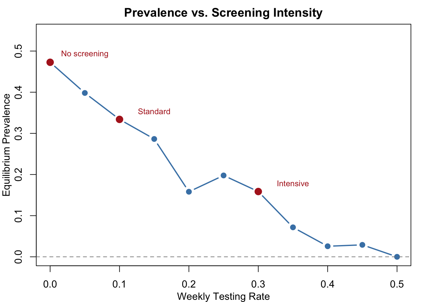

Figure 6: Dose-response curve showing equilibrium prevalence as a function of weekly testing rate. Red points mark the three named scenarios.

knitr::kable(data.frame(
  test.rate = test_rates,
  eq.prevalence = round(eq_prev, 3)
))

Table 2

test.rate	eq.prevalence
0.00	0.473
0.05	0.398
0.10	0.334
0.15	0.286
0.20	0.158
0.25	0.198
0.30	0.159
0.35	0.072
0.40	0.026
0.45	0.029
0.50	0.000

Parameters

Transmission

Parameter	Description	Default
`inf.prob`	Per-act transmission probability	0.4
`act.rate`	Acts per partnership per timestep	2

Recovery and Treatment

Parameter	Description	Default
`rec.rate`	Natural clearance rate (undiagnosed)	1/20 (mean ~20 weeks)
`rec.rate.tx`	Treatment recovery rate (diagnosed)	0.5 (mean ~2 weeks)

Screening

Parameter	Description	Varied
`test.rate`	Weekly testing rate for undiagnosed individuals	0 / 0.1 / 0.3
`test.dur`	Duration diagnosis persists (timesteps)	2

Network

Parameter	Description	Default
Population size	Number of nodes	500
Target edges	Mean concurrent partnerships	175
Concurrency	Nodes with degree > 1	110
Max degree	Upper bound on simultaneous partners	3
Partnership duration	Mean edge duration (weeks)	50

Module Execution Order

resim_nets → infection → tnt → recovery → prevalence

The tnt module runs after infection (so newly infected individuals can be tested in the same timestep) and before recovery (so newly diagnosed individuals immediately benefit from the higher treatment recovery rate).

Next Steps

Separate testing from treatment: Add a treatment uptake probability or delay between diagnosis and treatment initiation — not all diagnosed individuals start treatment immediately
Add partner notification / contact tracing: Diagnosed individuals’ partners receive expedited testing, amplifying the intervention’s reach
Risk-based screening: Vary test.rate by individual attributes (e.g., higher-risk groups test more frequently)
Add vital dynamics for longer-term STI modeling — see SI with Vital Dynamics
Model antimicrobial resistance: Introduce treatment failure or competing resistant strains — see Competing Strains
Extend to multi-stage disease: Model progression through disease stages with stage-dependent testing and treatment — see Syphilis
Add cost-effectiveness analysis: Attach costs to testing and treatment to evaluate intervention efficiency — see Cost-Effectiveness Analysis