flowchart LR
    S["<b>S</b><br/>Susceptible"] -->|"infection<br/>(main OR casual)"| A
    A["<b>Acute</b><br/>5x inf."] -->|"~12 wk"| C
    C["<b>Chronic</b><br/>1x inf."] -->|"~10 yr"| D["<b>AIDS</b><br/>2x inf."]
    D -->|"AIDS death"| out(( ))

    style S fill:#3498db,color:#fff
    style A fill:#e67e22,color:#fff
    style C fill:#e74c3c,color:#fff
    style D fill:#8e44ad,color:#fff
    style out fill:none,stroke:none
HIV Transmission with Care Cascade and PrEP
HIV
cascade
ART
PrEP
multilayer
advanced
Multilayer-network HIV model with a four-state care cascade (95-95-95) and PrEP, comparing treatment-as-prevention and pre-exposure prophylaxis.
Overview
A network HIV transmission model that compares the two prevention mechanisms at the center of 2025-2026 HIV policy: the treatment-as-prevention effect of a working care cascade (UNAIDS 95-95-95) and the susceptibility-reduction effect of pre-exposure prophylaxis (PrEP). The model brings together three EpiModel capabilities:
A two-layer partnership network. Main partnerships (long-duration, low-degree, high act rate) and casual partnerships (shorter-duration, lower-degree, lower act rate) are estimated as separate TERGMs that share the same node set. Both layers include a
concurrentERGM term, the structural feature most strongly implicated in generalized HIV spread (Morris & Kretzschmar 1997).An explicit care continuum. Every infected individual occupies one of four cascade states: undiagnosed, diagnosed (off ART), on ART but not yet suppressed, and virally suppressed. Transitions between states have separate, scenario-controlled rates that can reproduce the UNAIDS 95-95-95 targets and the leakage at each step.
PrEP as a risk-targeted, susceptibility-side intervention. PrEP is implemented as a per-edge reduction in acquisition probability for susceptibles, with stochastic initiation and discontinuation. Eligibility follows CDC behavioral-risk criteria: a node is indicated if either its total current degree (across the main and casual layers) is at or above a threshold, or it has at least one current HIV-positive partner. Efficacy is 95%, the high end of oral TDF/FTC and injectable cabotegravir / lenacapavir performance under consistent adherence.
The headline question: starting from a pre-treatment-era baseline, how much of the epidemic is averted by reaching UNAIDS 95-95-95, by rolling out PrEP at 50% coverage, and by combining the two?
TipDownload standalone scripts
- model.R — main simulation script
- module-fx.R — custom module functions
Model Structure
Disease Compartments
Disease progression is unidirectional, S to Acute to Chronic to AIDS. Each infected individual carries a separate cascade-state attribute.
| Compartment | status |
stage |
Description |
|---|---|---|---|
| Susceptible | "s" |
NA |
HIV-negative |
| Acute | "i" |
"acute" |
Recent infection; high viral load, ~5x infectiousness, ~12 weeks |
| Chronic | "i" |
"chronic" |
Long asymptomatic stage; reference infectiousness, ~10 years |
| AIDS | "i" |
"aids" |
Advanced disease; elevated mortality, ~2 years untreated |
A single Chronic stage is used because subdividing it into two stages with identical per-act transmissibility adds compartments without adding biology.
Care Cascade
Every PLHIV occupies one of four cascade states, defined by the joint values of diag.status, art.status, and vl.supp:
| State | diag.status |
art.status |
vl.supp |
Per-act infectiousness multiplier |
|---|---|---|---|---|
| Undiagnosed | 0 | 0 | 0 | 1 (full) |
| Diagnosed, off ART | 1 | 0 | 0 | 1 (full) |
| On ART, not yet suppressed | 1 | 1 | 0 | 0.30 |
| Virally suppressed (U=U) | 1 | 1 | 1 | 0.01 (essentially zero) |
The U=U value (0.01) reflects HPTN 052 and PARTNER trial evidence that durable viral suppression on ART eliminates sexual transmission. The intermediate 0.30 multiplier represents the 2-3 month ramp from ART initiation to undetectable plasma viral load.
Flow Diagram
Within each infected stage, the four cascade states are connected by:
flowchart LR
    U["<b>Undiagnosed</b>"] -->|"test.rate<br/>(aids.dx.rate)"| D["<b>Diagnosed</b><br/>off ART"]
    D -->|"linkage.rate (initial)<br/>art.reinit.rate (re-engagement)"| A["<b>On ART</b><br/>unsuppressed"]
    A -->|"suppression.rate"| V["<b>Suppressed</b><br/>U=U"]
    A -->|"art.disc.rate"| D
    V -->|"art.disc.rate"| D

    style U fill:#7f8c8d,color:#fff
    style D fill:#e74c3c,color:#fff
    style A fill:#f39c12,color:#fff
    style V fill:#27ae60,color:#fff
AIDS-stage infections receive a higher aids.dx.rate to represent symptom-driven presentation to care. Nodes that discontinue ART return to the Diagnosed off ART state with their prior art.time retained, so subsequent re-engagement uses the (typically lower) art.reinit.rate rather than the initial linkage.rate — reflecting the empirical pattern that re-engagement after disengagement is slower than initial linkage.
Setup
suppressMessages(library(EpiModel))

N <- 1500
nsims <- 5
ncores <- 5
nsteps <- 1040          # 20 years on a weekly timestep
departure_rate <- 0.0005
Network Layers
Both layers are estimated as separate ERGMs that share the same node set. Both include a concurrent term to encode overlapping partnerships, the structural feature most strongly implicated in generalized HIV spread.
Main partnership layer
Long-duration ties (200 weeks ~ 4 years), low mean degree (~0.5), with mild concurrency. A degrange(from = 3) term caps the distribution at 2 simultaneous main partners — 3+ concurrent main partnerships is not a plausible main-partnership structure.
nw <- network_initialize(N)

mean_deg_main <- 0.5
concurrent_main <- round(0.04 * N)    # ~4% of nodes have 2+ main partners
formation_main <- ~edges + concurrent + degrange(from = 3)
1target_main <- c(mean_deg_main * N / 2, concurrent_main, 0)
diss_main <- dissolution_coefs(~offset(edges), duration = 200,
                               d.rate = departure_rate)

est_main <- netest(nw, formation_main, target_main, diss_main,
verbose = FALSE)- 1
-
Target statistics: total edges, count of concurrent (degree 2+) nodes, and zero nodes with degree 3+ (the
degrange(from = 3)term caps the distribution).
Casual partnership layer
Shorter ties (26 weeks ~ 6 months), lower mean degree (~0.3), with concurrency lifted ~2.7x above the Poisson baseline (1 - exp(-0.3) * 1.3 = 3.7%) by the concurrent term. The upper tail of casual degree is deliberately not capped: the small set of nodes with many concurrent casual ties is the high-activity subgroup that drives a disproportionate share of transmission and motivates targeted PrEP. Truncating it with degrange() would erase the structural heterogeneity the intervention is designed to address.
mean_deg_cas <- 0.3
concurrent_cas <- round(0.10 * N)     # ~10% have 2+ casual partners
1formation_cas <- ~edges + concurrent
target_cas <- c(mean_deg_cas * N / 2, concurrent_cas)
diss_cas <- dissolution_coefs(~offset(edges), duration = 26,
                              d.rate = departure_rate)

est_cas <- netest(nw, formation_cas, target_cas, diss_cas,
verbose = FALSE)- 1
-
No
degrange()constraint on the casual layer: the right tail of casual degree is the high-activity subgroup that drives transmission and is the natural PrEP target. Theprep()module flags nodes with high total degree (across the two layers) as PrEP-indicated, so leaving this tail unconstrained is what lets risk-based targeting do work.
Custom Modules
Progression Module
Acute to Chronic to AIDS, using a snapshot of stage at function entry so no individual cascades through two stages in a single timestep, regardless of progression rate. The first call also initializes every custom attribute used by the cascade and PrEP modules; this is done inline rather than via a separate init module so the helper is serialized into each parallel worker along with progress() itself.
progress <- function(dat, at) {

  # ---- Attribute initializer (runs once on first call) ----
  if (is.null(get_attr(dat, "stage", override.null.error = TRUE))) {
    n <- length(get_attr(dat, "active"))
    .active <- get_attr(dat, "active")
    .status <- get_attr(dat, "status")

    # Seed-infected stage distribution proportional to mean stage
    # duration (acute 12 wk, chronic 520 wk, AIDS 104 wk) -- avoids
1    # a synchronous cohort wave from starting everyone as acute.
    stage0_init <- rep(NA_character_, n)
    stage.time0_init <- rep(NA_integer_, n)
    inf_ids <- which(.active == 1 & .status == "i")
    if (length(inf_ids) > 0) {
      durs <- c(acute = 12, chronic = 520, aids = 104)
      probs <- durs / sum(durs)
      stage0_init[inf_ids] <- sample(names(probs), length(inf_ids),
                                     replace = TRUE, prob = probs)
      stage.time0_init[inf_ids] <- 0L
    }

    dat <- set_attr(dat, "stage", stage0_init)
    dat <- set_attr(dat, "stage.time", stage.time0_init)
    dat <- set_attr(dat, "diag.status", rep(0L, n))
    dat <- set_attr(dat, "art.status", rep(0L, n))
    dat <- set_attr(dat, "vl.supp", rep(0L, n))
    dat <- set_attr(dat, "art.time", rep(NA_integer_, n))
    # prep.status starts NA; prep() runs after progress() and replaces NA
    # values with an indication-based sample once the network is available.
    dat <- set_attr(dat, "prep.status", rep(NA_integer_, n))
  }

  active <- get_attr(dat, "active")
  stage <- get_attr(dat, "stage")
  stage.time <- get_attr(dat, "stage.time")
  art.status <- get_attr(dat, "art.status")
  vl.supp <- get_attr(dat, "vl.supp")
  infTime <- get_attr(dat, "infTime")

  acute.to.chronic.rate <- get_param(dat, "acute.to.chronic.rate")
  chronic.to.aids.rate <- get_param(dat, "chronic.to.aids.rate")
  art.prog.mult <- get_param(dat, "art.prog.mult")

2  stage0 <- stage
  in_stage <- !is.na(stage.time) & active == 1
  stage.time[in_stage] <- stage.time[in_stage] + 1L

  ## Acute -> Chronic
  ids_ac <- which(active == 1 & !is.na(stage0) & stage0 == "acute" &
3                    !is.na(infTime) & infTime < at)
  n_ac <- 0
  if (length(ids_ac) > 0) {
    supp <- art.status[ids_ac] == 1 & vl.supp[ids_ac] == 1
    rates <- ifelse(supp, acute.to.chronic.rate * art.prog.mult,
                          acute.to.chronic.rate)
    hits <- rbinom(length(ids_ac), 1, rates) == 1
    new_chronic <- ids_ac[hits]
    if (length(new_chronic) > 0) {
      stage[new_chronic] <- "chronic"
      stage.time[new_chronic] <- 0L
      n_ac <- length(new_chronic)
    }
  }

  ## Chronic -> AIDS
  ids_ca <- which(active == 1 & !is.na(stage0) & stage0 == "chronic")
  n_ca <- 0
  if (length(ids_ca) > 0) {
    supp <- art.status[ids_ca] == 1 & vl.supp[ids_ca] == 1
    rates <- ifelse(supp, chronic.to.aids.rate * art.prog.mult,
                          chronic.to.aids.rate)
    hits <- rbinom(length(ids_ca), 1, rates) == 1
    new_aids <- ids_ca[hits]
    if (length(new_aids) > 0) {
      stage[new_aids] <- "aids"
      stage.time[new_aids] <- 0L
      n_ca <- length(new_aids)
    }
  }

  dat <- set_attr(dat, "stage", stage)
  dat <- set_attr(dat, "stage.time", stage.time)

  is_act <- active == 1
  dat <- set_epi(dat, "ac.flow", at, n_ac)
  dat <- set_epi(dat, "ca.flow", at, n_ca)
  dat <- set_epi(dat, "acute.num", at, sum(is_act & stage %in% "acute"))
  dat <- set_epi(dat, "chronic.num", at, sum(is_act & stage %in% "chronic"))
  dat <- set_epi(dat, "aids.num", at, sum(is_act & stage %in% "aids"))

  return(dat)
}- 1
- Seed-infected nodes are sampled across stages in proportion to mean stage duration, so the initial population approximates the stage-equilibrium distribution rather than entering as a synchronized acute cohort that would otherwise produce artifactual waves moving through chronic and AIDS together.
- 2
-
Snapshot of
stageat function entry. All eligibility checks below read fromstage0, so a node cannot cascade through two stages within one step. - 3
-
infTime < atexcludes brand-new infections (written byinfect()earlier in this step) so the acute period is always at least one timestep regardless ofacute.to.chronic.rate.
Cascade Module
The four-state care continuum. Each timestep moves one cascade step per individual at most (snapshot pattern).
cascade <- function(dat, at) {

  active <- get_attr(dat, "active")
  status <- get_attr(dat, "status")
  stage <- get_attr(dat, "stage")
  diag.status <- get_attr(dat, "diag.status")
  art.status <- get_attr(dat, "art.status")
  vl.supp <- get_attr(dat, "vl.supp")
  art.time <- get_attr(dat, "art.time")

  test.rate <- get_param(dat, "test.rate")
  aids.dx.rate <- get_param(dat, "aids.dx.rate")
  linkage.rate <- get_param(dat, "linkage.rate")
  art.reinit.rate <- get_param(dat, "art.reinit.rate")
  suppression.rate <- get_param(dat, "suppression.rate")
  art.disc.rate <- get_param(dat, "art.disc.rate")

  diag0 <- diag.status
  art0 <- art.status
  supp0 <- vl.supp
  is_inf <- active == 1 & status == "i"

  ## 1. Testing: undiagnosed -> diagnosed
  ids_undx <- which(is_inf & diag0 == 0)
  if (length(ids_undx) > 0) {
    rates <- ifelse(!is.na(stage[ids_undx]) & stage[ids_undx] == "aids",
1                    aids.dx.rate, test.rate)
    hits <- rbinom(length(ids_undx), 1, rates) == 1
    new_dx <- ids_undx[hits]
    if (length(new_dx) > 0) diag.status[new_dx] <- 1L
  }

  ## 2a. Linkage: newly-diagnosed (no prior ART history) -> on ART
  ids_link_new <- which(is_inf & diag0 == 1 & art0 == 0 &
2                          is.na(art.time))
  if (length(ids_link_new) > 0) {
    hits <- rbinom(length(ids_link_new), 1, linkage.rate) == 1
    new_art <- ids_link_new[hits]
    if (length(new_art) > 0) {
      art.status[new_art] <- 1L
      art.time[new_art] <- at
    }
  }

  ## 2b. Re-engagement: previously-on-ART -> on ART at art.reinit.rate
  ids_link_re <- which(is_inf & diag0 == 1 & art0 == 0 &
                         !is.na(art.time))
  if (length(ids_link_re) > 0) {
    hits <- rbinom(length(ids_link_re), 1, art.reinit.rate) == 1
    reinit <- ids_link_re[hits]
    if (length(reinit) > 0) {
      art.status[reinit] <- 1L
      art.time[reinit] <- at
    }
  }

  ## 3. Suppression: on ART, not yet suppressed -> suppressed
  ids_sup <- which(is_inf & art0 == 1 & supp0 == 0)
  if (length(ids_sup) > 0) {
    hits <- rbinom(length(ids_sup), 1, suppression.rate) == 1
    new_supp <- ids_sup[hits]
    if (length(new_supp) > 0) vl.supp[new_supp] <- 1L
  }

  ## 4. Discontinuation: on ART -> off ART (clears suppression too)
  ids_disc <- which(is_inf & art0 == 1)
  if (length(ids_disc) > 0) {
    hits <- rbinom(length(ids_disc), 1, art.disc.rate) == 1
    disc <- ids_disc[hits]
    if (length(disc) > 0) {
      art.status[disc] <- 0L
3      vl.supp[disc] <- 0L
    }
  }

  dat <- set_attr(dat, "diag.status", diag.status)
  dat <- set_attr(dat, "art.status", art.status)
  dat <- set_attr(dat, "vl.supp", vl.supp)
  dat <- set_attr(dat, "art.time", art.time)

  dat <- set_epi(dat, "dx.flow", at, sum(diag.status == 1 & diag0 == 0))
  dat <- set_epi(dat, "link.flow", at, sum(art.status == 1 & art0 == 0))
  dat <- set_epi(dat, "supp.flow", at, sum(vl.supp == 1 & supp0 == 0))
  dat <- set_epi(dat, "disc.flow", at, sum(art.status == 0 & art0 == 1))
  dat <- set_epi(dat, "dx.num", at, sum(is_inf & diag.status == 1))
  dat <- set_epi(dat, "art.num", at, sum(is_inf & art.status == 1))
  dat <- set_epi(dat, "supp.num", at, sum(is_inf & vl.supp == 1))

  return(dat)
}- 1
-
AIDS-stage infections are diagnosed at the higher
aids.dx.rateto represent symptom-driven presentation to care (around 20-week mean time to diagnosis from AIDS onset, vs. ~67 weeks of background screening for acute/chronic). - 2
-
The split between
linkage.rate(initial linkage) andart.reinit.rate(re-engagement after a prior ART episode) usesart.timeas the history flag:NAmeans the node has never been on ART; non-NAmeans they have, so a slower re-engagement rate applies. Discontinuation leavesart.timeintact precisely so this distinction is preserved. - 3
- Discontinuation clears both the ART flag and the suppression flag, returning the node to the diagnosed-off-ART state. Re-engagement next step uses the path described in note 2.
PrEP Module
PrEP turnover among indicated HIV-negative individuals. The indicated set is recomputed every step as the union of two CDC behavioral-risk criteria: total current degree (across both layers) at or above prep.indic.deg, and a current HIV+ partner. Initiation applies only to indicated susceptibles; discontinuation applies to all current users regardless of indication (real-world drop-off is driven by adherence and access more than by indication change). PrEP is cleared on HIV acquisition by infect().
prep <- function(dat, at) {

  active <- get_attr(dat, "active")
  status <- get_attr(dat, "status")
  prep.status <- get_attr(dat, "prep.status")

  prep.init.cov <- get_param(dat, "prep.init.cov")
  prep.start.rate <- get_param(dat, "prep.start.rate")
  prep.stop.rate <- get_param(dat, "prep.stop.rate")
  prep.indic.deg <- get_param(dat, "prep.indic.deg")

  ## Compute indication: high total degree OR HIV+ partner
  n <- length(active)
  total_deg <- integer(n)
  has_pos_partner <- logical(n)
  for (k in 1:2) {
    el <- get_edgelist(dat, network = k)
    if (is.null(el) || nrow(el) == 0) next
1    total_deg <- total_deg + get_degree(el)
    has_pos_partner[el[, 2][status[el[, 1]] == "i"]] <- TRUE
    has_pos_partner[el[, 1][status[el[, 2]] == "i"]] <- TRUE
  }
  indicated <- active == 1 & status == "s" &
               (total_deg >= prep.indic.deg | has_pos_partner)

  ## First-call initialization (NA prep.status from progress's init block)
  needs_init <- is.na(prep.status) & active == 1
  if (any(needs_init)) {
    prep.status[needs_init] <- 0L
    if (prep.init.cov > 0) {
      ids_init <- which(needs_init & indicated)
      if (length(ids_init) > 0) {
        prep.status[ids_init] <- rbinom(length(ids_init), 1,
2                                        prep.init.cov)
      }
    }
  }

  ## Initiation: only among indicated susceptibles
  if (prep.start.rate > 0) {
    ids_off <- which(indicated & prep.status == 0)
    if (length(ids_off) > 0) {
      hits <- rbinom(length(ids_off), 1, prep.start.rate) == 1
      prep.status[ids_off[hits]] <- 1L
    }
  }

  ## Discontinuation: applies to all PrEP users regardless of indication
  if (prep.stop.rate > 0) {
    ids_on <- which(active == 1 & status == "s" & prep.status == 1)
    if (length(ids_on) > 0) {
      hits <- rbinom(length(ids_on), 1, prep.stop.rate) == 1
      prep.status[ids_on[hits]] <- 0L
    }
  }

  dat <- set_attr(dat, "prep.status", prep.status)

  is_sus <- active == 1 & status == "s"
  dat <- set_epi(dat, "prep.num", at, sum(is_sus & prep.status == 1))
3  dat <- set_epi(dat, "prep.indic.num", at, sum(indicated))
  dat <- set_epi(dat, "prep.num.indic", at,
                 sum(indicated & prep.status == 1))

  return(dat)
}- 1
-
get_degree(el)tabulates each node’s edge endpoints on the current layer; summing acrossk = 1:2gives total degree across the main and casual layers. - 2
- Initial coverage is sampled only among nodes that meet the indication criteria in the first step’s network. Without this, the PrEP scenario would start with population-wide coverage and then need to “shed” non-indicated users over many timesteps.
- 3
-
Tracking
prep.indic.numseparately lets the analysis distinguish coverage among indicated susceptibles (the policy-relevant denominator) from coverage among all susceptibles (the population-level metric).
Infection Module
Multilayer transmission. Walks discord_edgelist() for each layer and computes per-act and per-partnership-per-week probabilities. Susceptible-side PrEP and the infector’s cascade state both modify the per-act probability.
infect <- function(dat, at) {

  active <- get_attr(dat, "active")
  status <- get_attr(dat, "status")
  stage <- get_attr(dat, "stage")
  art.status <- get_attr(dat, "art.status")
  vl.supp <- get_attr(dat, "vl.supp")
  prep.status <- get_attr(dat, "prep.status")
  infTime <- get_attr(dat, "infTime")
  stage.time <- get_attr(dat, "stage.time")

  inf.prob.act <- get_param(dat, "inf.prob.act")
  rel.inf.acute <- get_param(dat, "rel.inf.acute")
  rel.inf.aids <- get_param(dat, "rel.inf.aids")
  rel.inf.art.unsupp <- get_param(dat, "rel.inf.art.unsupp")
  rel.inf.art.supp <- get_param(dat, "rel.inf.art.supp")
  prep.efficacy <- get_param(dat, "prep.efficacy")
  acts.main <- get_param(dat, "acts.main")
  acts.casual <- get_param(dat, "acts.casual")

  layer_acts <- c(acts.main, acts.casual)
  all_new <- integer(0)

  for (k in 1:2) {
1    del <- discord_edgelist(dat, at, network = k)
    if (is.null(del) || nrow(del) == 0) next

    stg <- stage[del$inf]
    art <- art.status[del$inf]
    sup <- vl.supp[del$inf]

    stage_mult <- ifelse(!is.na(stg) & stg == "acute", rel.inf.acute,
2                  ifelse(!is.na(stg) & stg == "aids",  rel.inf.aids, 1))
    art_mult <- ifelse(art == 1 & sup == 1, rel.inf.art.supp,
3                ifelse(art == 1 & sup == 0, rel.inf.art.unsupp, 1))

    p_act <- inf.prob.act * stage_mult * art_mult
    p_act <- p_act * ifelse(prep.status[del$sus] == 1,
4                            1 - prep.efficacy, 1)
    p_act <- pmax(pmin(p_act, 1), 0)

5    p_edge <- 1 - (1 - p_act)^layer_acts[k]

    transmit <- rbinom(length(p_edge), 1, p_edge) == 1
    if (any(transmit)) all_new <- c(all_new, del$sus[transmit])
  }

  all_new <- unique(all_new)
  n_new <- length(all_new)

  if (n_new > 0) {
    status[all_new] <- "i"
    stage[all_new] <- "acute"
    stage.time[all_new] <- 0L
    infTime[all_new] <- at
6    prep.status[all_new] <- 0L

    dat <- set_attr(dat, "status", status)
    dat <- set_attr(dat, "stage", stage)
    dat <- set_attr(dat, "stage.time", stage.time)
    dat <- set_attr(dat, "infTime", infTime)
    dat <- set_attr(dat, "prep.status", prep.status)
  }

  dat <- set_epi(dat, "si.flow", at, n_new)
  return(dat)
}- 1
-
discord_edgelist(dat, at, network = k)returns one row per active S-I edge on layerk, withsusandinfcolumns. Looping overkin1:2handles both layers. - 2
- Stage multiplier on the infector side: acute is 5x, AIDS is 2x, chronic is 1x.
- 3
- ART multiplier: virally suppressed is 0.01 (U=U), on ART but not yet suppressed is 0.30, off ART is 1.
- 4
-
Susceptible-side PrEP cuts the per-act probability by
1 - prep.efficacy. - 5
- Per-act probability is converted to per-partnership-per-week via the standard formula.
- 6
- PrEP is cleared on seroconversion so the prep.num statistic reflects HIV-negative users only.
Departure Module
Background departure for everyone (a constant per-capita rate) plus an elevated AIDS-related rate. Suppressive ART extends AIDS survival by art.aids.surv.mult (default 10x).
dfunc <- function(dat, at) {

  active <- get_attr(dat, "active")
  stage <- get_attr(dat, "stage")
  art.status <- get_attr(dat, "art.status")
  vl.supp <- get_attr(dat, "vl.supp")
  exitTime <- get_attr(dat, "exitTime")

  departure.rate <- get_param(dat, "departure.rate")
  aids.depart.rate <- get_param(dat, "aids.depart.rate")
  art.aids.surv.mult <- get_param(dat, "art.aids.surv.mult")

  ids_bg <- which(active == 1 & (is.na(stage) | stage != "aids"))
  bg_dep <- ids_bg[rbinom(length(ids_bg), 1, departure.rate) == 1]

  ids_aids <- which(active == 1 & !is.na(stage) & stage == "aids")
  aids_dep <- integer(0)
  if (length(ids_aids) > 0) {
    on_supp <- art.status[ids_aids] == 1 & vl.supp[ids_aids] == 1
    rates <- ifelse(on_supp, aids.depart.rate * art.aids.surv.mult,
1                             aids.depart.rate)
    aids_dep <- ids_aids[rbinom(length(ids_aids), 1, rates) == 1]
  }

  all_dep <- c(bg_dep, aids_dep)
  if (length(all_dep) > 0) {
    active[all_dep] <- 0L
    exitTime[all_dep] <- at
    dat <- set_attr(dat, "active", active)
    dat <- set_attr(dat, "exitTime", exitTime)
  }

  dat <- set_epi(dat, "dep.flow", at, length(all_dep))
  dat <- set_epi(dat, "aids.dep.flow", at, length(aids_dep))
  return(dat)
}- 1
-
ART suppression reduces AIDS mortality 10-fold (default
art.aids.surv.mult = 0.1), reflecting the survival benefit of effective HIV therapy initiated even in late-stage disease.
Arrival Module
New susceptibles arrive at a per-capita Poisson rate. Each custom attribute is extended via append_attr() to stay in lockstep with the EpiModel core attributes.
afunc <- function(dat, at) {
  active <- get_attr(dat, "active")
  a.rate <- get_param(dat, "arrival.rate")
  nArr <- rpois(1, sum(active == 1) * a.rate)

  if (nArr > 0) {
1    dat <- append_core_attr(dat, at, nArr)
    dat <- append_attr(dat, "status", "s", nArr)
    dat <- append_attr(dat, "stage", NA_character_, nArr)
    dat <- append_attr(dat, "stage.time", NA_integer_, nArr)
    dat <- append_attr(dat, "infTime", NA_integer_, nArr)
    dat <- append_attr(dat, "diag.status", 0L, nArr)
    dat <- append_attr(dat, "art.status", 0L, nArr)
    dat <- append_attr(dat, "vl.supp", 0L, nArr)
    dat <- append_attr(dat, "art.time", NA_integer_, nArr)
    dat <- append_attr(dat, "prep.status", 0L, nArr)
  }

  dat <- set_epi(dat, "arr.flow", at, nArr)
  return(dat)
}- 1
-
append_core_attr()extends the EpiModel-managed core attributes (active,entrTime,exitTime,unique_ids). The subsequentappend_attr()calls extend each of our custom attribute vectors by the same number of entries.
Epidemic Simulation
Base Parameters
Stage and ART-status multipliers reflect viral-load biology and the U=U evidence base; PrEP efficacy reflects the high end of demonstrated effectiveness with consistent adherence (oral TDF/FTC, injectable CAB-LA, lenacapavir). The base parameter object holds every parameter the modules read; cascade and PrEP rates are defaulted to zero so the “no intervention” scenario inherits an all-off baseline directly from this set.
param_base <- param.net(
  # Transmission biology
  inf.prob.act = 0.0025,
  rel.inf.acute = 5,
  rel.inf.aids = 2,
  rel.inf.art.unsupp = 0.30,
  rel.inf.art.supp = 0.01,
  prep.efficacy = 0.95,
  acts.main = 3,
  acts.casual = 1,
  # Disease progression (per week)
  acute.to.chronic.rate = 1 / 12,
  chronic.to.aids.rate = 1 / 520,
  aids.depart.rate = 1 / 104,
  art.prog.mult = 0.5,
  art.aids.surv.mult = 0.1,
  # Care cascade (off by default)
  test.rate = 0,
  aids.dx.rate = 0,
  linkage.rate = 0,
  art.reinit.rate = 0,
  suppression.rate = 0,
  art.disc.rate = 0,
  # PrEP (off by default; indication threshold set up front)
  prep.init.cov = 0,
  prep.start.rate = 0,
  prep.stop.rate = 0,
  prep.indic.deg = 2,
  # Vital dynamics
  departure.rate = departure_rate,
  arrival.rate = 0.00065
)

init <- init.net(i.num = round(0.08 * N))
Control Settings
control <- control.net(
  type = NULL,
  nsims = nsims,
  ncores = ncores,
  nsteps = nsteps,
  tergmLite = TRUE,
  resimulate.network = TRUE,
  infection.FUN = infect,
  progress.FUN = progress,
  cascade.FUN = cascade,
  prep.FUN = prep,
  departures.FUN = dfunc,
  arrivals.FUN = afunc,
  verbose = FALSE
)
Scenarios
Scenarios are defined as a flat data frame (one row per scenario, columns matching parameter names in param_base) and converted to a scenario list with create_scenario_list(). Inside the loop, use_scenario(param_base, scn) returns a parameter object with the scenario’s row applied to the base defaults. The .scenario.id column labels each scenario; .at = 0 applies the override before step 1.
scenarios.df <- data.frame(
  .scenario.id     = c("none", "cascade", "prep",  "both"),
  .at              = 0,
  test.rate        = c(0,       0.015,     0,       0.015),
  aids.dx.rate     = c(0,       0.050,     0,       0.050),
  linkage.rate     = c(0,       0.100,     0,       0.100),
  art.reinit.rate  = c(0,       0.030,     0,       0.030),
  suppression.rate = c(0,       1 / 12,    0,       1 / 12),
  art.disc.rate    = c(0,       0.002,     0,       0.002),
  prep.init.cov    = c(0,       0,         0.50,    0.50),
  prep.start.rate  = c(0,       0,         0.015,   0.015),
  prep.stop.rate   = c(0,       0,         0.015,   0.015)
)
scenarios.list <- create_scenario_list(scenarios.df)

labels <- c(none = "No intervention",
            cascade = "Cascade (95-95-95)",
            prep = "PrEP (50% coverage)",
            both = "Cascade + PrEP")

sims <- list()
for (scn in scenarios.list) {
  sims[[scn$id]] <- netsim(list(est_main, est_cas),
                           use_scenario(param_base, scn),
                           init, control)
}
Derived Measures
for (s in names(sims)) {
  sims[[s]] <- mutate_epi(sims[[s]],
    prev = i.num / num,
    ir100py = 52 * 100 * si.flow / s.num,
    pct.dx = dx.num / i.num,
    pct.art = art.num / i.num,
    pct.supp = supp.num / i.num,
    prep.cov = prep.num / s.num
  )
}
Analysis
HIV Prevalence by Scenario
The headline outcome: only a working care cascade bends the prevalence curve downward over a 20-year horizon. PrEP slows but does not reverse the epidemic in this parameterization; the combined intervention is closest to elimination.
cols_scn <- c(none = "firebrick", cascade = "steelblue",
              prep = "darkorange", both = "darkgreen")

par(mfrow = c(1, 1), mar = c(4, 4, 2.5, 1), mgp = c(2.5, 0.8, 0))
prev_max <- max(sapply(sims, function(s) {
  df <- as.data.frame(s); max(df$prev, na.rm = TRUE)
}))
plot(sims[[1]], y = "prev",
     main = "HIV Prevalence by Scenario",
     ylab = "Prevalence", xlab = "Week",
     mean.col = cols_scn[1], mean.lwd = 2, mean.smooth = TRUE,
     qnts = FALSE, legend = FALSE,
     ylim = c(0, 1.05 * prev_max))
for (i in 2:length(sims)) {
  plot(sims[[i]], y = "prev", add = TRUE,
       mean.col = cols_scn[i], mean.lwd = 2, mean.smooth = TRUE,
       qnts = FALSE, legend = FALSE)
}
legend("topleft", legend = labels, col = cols_scn, lwd = 2,
       bty = "n", cex = 0.9)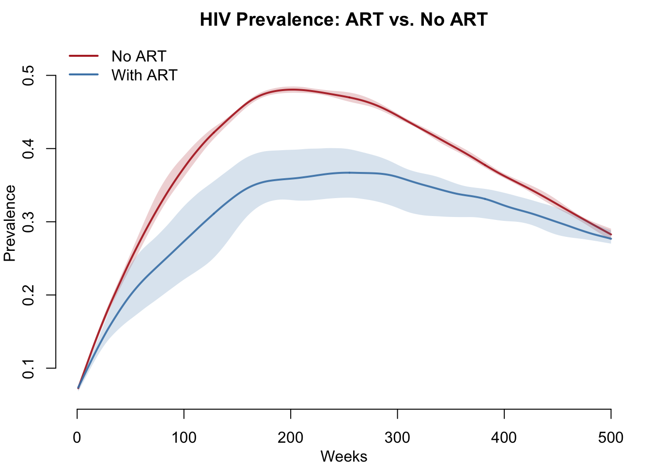
HIV Incidence Rate
New infections per 100 person-years per scenario. The cascade and combined scenarios drive incidence near zero; PrEP holds incidence at a reduced level but does not eliminate it.
par(mfrow = c(1, 1), mar = c(4, 4, 2.5, 1), mgp = c(2.5, 0.8, 0))
inc_max <- max(sapply(sims, function(s) {
  df <- as.data.frame(s); max(df$ir100py, na.rm = TRUE)
}))
plot(sims[[1]], y = "ir100py",
     main = "HIV Incidence Rate by Scenario",
     ylab = "New infections per 100 person-years",
     xlab = "Week",
     mean.col = cols_scn[1], mean.lwd = 2, mean.smooth = TRUE,
     qnts = FALSE, legend = FALSE,
     ylim = c(0, 1.05 * inc_max))
for (i in 2:length(sims)) {
  plot(sims[[i]], y = "ir100py", add = TRUE,
       mean.col = cols_scn[i], mean.lwd = 2, mean.smooth = TRUE,
       qnts = FALSE, legend = FALSE)
}
legend("topright", legend = labels, col = cols_scn, lwd = 2,
       bty = "n", cex = 0.9)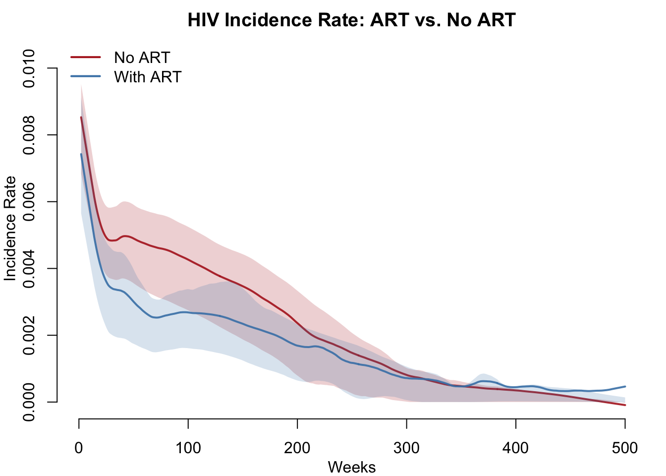
Care Cascade Attainment
The cascade scenario reaches the UNAIDS 95-95-95 targets at equilibrium: ~98% of PLHIV diagnosed, ~92% on ART, ~89% virally suppressed. The dashed gray lines mark the cumulative targets (95%, 90.25%, 85.7% of all PLHIV). Only the cascade scenario is shown here because the “both” scenario uses identical cascade parameters and reaches identical attainment.
par(mfrow = c(1, 1), mar = c(4, 4, 2.5, 1), mgp = c(2.5, 0.8, 0))
plot(sims[["cascade"]], y = "pct.dx",
     main = "Care Cascade Attainment (cascade scenario)",
     ylab = "Fraction of PLHIV", xlab = "Week",
     mean.col = "steelblue", mean.lwd = 2, mean.smooth = TRUE,
     qnts = FALSE, legend = FALSE, ylim = c(0, 1))
plot(sims[["cascade"]], y = "pct.art", add = TRUE,
     mean.col = "darkorange", mean.lwd = 2, mean.smooth = TRUE,
     qnts = FALSE, legend = FALSE)
plot(sims[["cascade"]], y = "pct.supp", add = TRUE,
     mean.col = "darkgreen", mean.lwd = 2, mean.smooth = TRUE,
     qnts = FALSE, legend = FALSE)
abline(h = c(0.95, 0.95 ^ 2, 0.95 ^ 3), lty = 3, col = "gray50")
legend("bottomright",
       legend = c("% Diagnosed", "% on ART", "% Suppressed",
                  "UNAIDS 95-95-95 targets"),
       col = c("steelblue", "darkorange", "darkgreen", "gray50"),
       lwd = c(2, 2, 2, 1), lty = c(1, 1, 1, 3),
       bty = "n", cex = 0.9)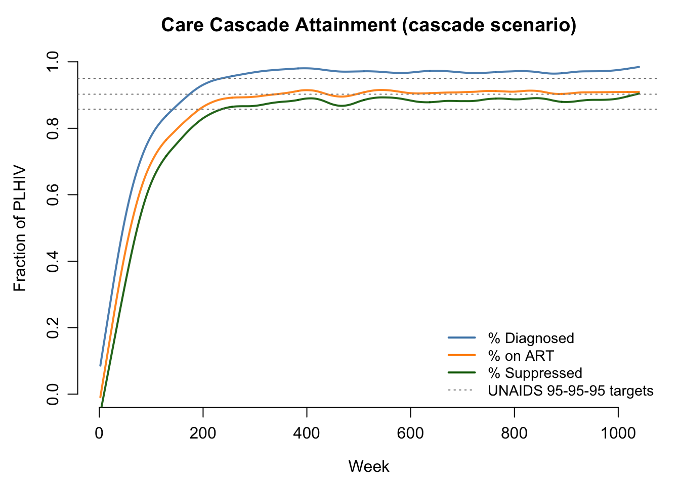
PrEP Coverage Among Indicated vs. All Susceptibles
The PrEP scenario uses risk-based eligibility (total degree >= 2 OR HIV+ partner). At equilibrium, ~50% of indicated susceptibles are on PrEP (solid line); population-wide coverage is much lower (dashed line) because the indicated subset is only a fraction of all susceptibles. The contrast is the point of the targeting design: by concentrating doses on the indicated group, the intervention achieves substantial impact without offering PrEP to everyone.
sims[["prep"]] <- mutate_epi(sims[["prep"]],
  prep.cov.indic = prep.num.indic / prep.indic.num)
par(mfrow = c(1, 1), mar = c(4, 4, 2.5, 1), mgp = c(2.5, 0.8, 0))
plot(sims[["prep"]], y = "prep.cov.indic",
     main = "PrEP Coverage Among Indicated vs. All Susceptibles",
     ylab = "Fraction on PrEP", xlab = "Week",
     mean.col = "darkorange", mean.lwd = 2, mean.smooth = TRUE,
     qnts = FALSE, legend = FALSE, ylim = c(0, 1))
plot(sims[["prep"]], y = "prep.cov", add = TRUE,
     mean.col = "darkorange", mean.lwd = 2, mean.smooth = TRUE,
     mean.lty = 2, qnts = FALSE, legend = FALSE)
legend("topright",
       legend = c("Indicated susceptibles (target population)",
                  "All susceptibles (population coverage)"),
       col = c("darkorange", "darkorange"),
       lwd = 2, lty = c(1, 2), bty = "n", cex = 0.9)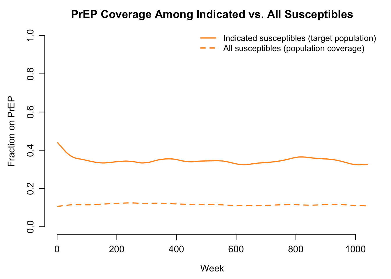
Summary Table
df_summary <- function(s) {
  df <- as.data.frame(sims[[s]])
  last_t <- max(df$time)
  late <- df$time >= 0.5 * last_t
  data.frame(
    Scenario = labels[s],
    Cum_infections = round(sum(df$si.flow, na.rm = TRUE) / nsims),
    Final_prev = round(mean(df$prev[df$time == last_t], na.rm = TRUE), 3),
    Mean_inc_100py = round(mean(df$ir100py[late], na.rm = TRUE), 2),
    Pct_diagnosed = round(100 * mean(df$pct.dx[late], na.rm = TRUE), 1),
    Pct_on_ART = round(100 * mean(df$pct.art[late], na.rm = TRUE), 1),
    Pct_suppressed = round(100 * mean(df$pct.supp[late], na.rm = TRUE), 1),
    stringsAsFactors = FALSE
  )
}
summary_tbl <- do.call(rbind, lapply(names(sims), df_summary))
summary_tbl$Infections_averted <-
  summary_tbl$Cum_infections[1] - summary_tbl$Cum_infections
knitr::kable(summary_tbl, row.names = FALSE)| Scenario | Cum_infections | Final_prev | Mean_inc_100py | Pct_diagnosed | Pct_on_ART | Pct_suppressed | Infections_averted |
|---|---|---|---|---|---|---|---|
| No intervention | 477 | 0.156 | 1.91 | 0.0 | 0.0 | 0.0 | 0 |
| Cascade (95-95-95) | 79 | 0.051 | 0.15 | 97.0 | 90.9 | 88.6 | 398 |
| PrEP (50% coverage) | 228 | 0.062 | 0.69 | 0.0 | 0.0 | 0.0 | 249 |
| Cascade + PrEP | 42 | 0.038 | 0.07 | 98.6 | 92.1 | 89.6 | 435 |
Parameters Reference
Transmission biology
| Parameter | Description | Default |
|---|---|---|
inf.prob.act |
Per-act transmission probability (chronic, off-ART reference) | 0.0025 |
rel.inf.acute |
Acute-stage infectiousness multiplier | 5 |
rel.inf.aids |
AIDS-stage infectiousness multiplier | 2 |
rel.inf.art.unsupp |
Multiplier on ART, not yet suppressed | 0.30 |
rel.inf.art.supp |
Multiplier while suppressed (U=U) | 0.01 |
prep.efficacy |
Per-edge susceptibility reduction on PrEP | 0.95 |
acts.main |
Acts per main partnership per week | 3 |
acts.casual |
Acts per casual partnership per week | 1 |
Disease progression (per week)
| Parameter | Description | Default |
|---|---|---|
acute.to.chronic.rate |
Acute to Chronic | 1/12 (~12 weeks) |
chronic.to.aids.rate |
Chronic to AIDS | 1/520 (~10 years) |
aids.depart.rate |
AIDS-stage mortality | 1/104 (~2 years untreated) |
art.prog.mult |
Multiplier on progression while suppressed | 0.5 |
art.aids.surv.mult |
Multiplier on AIDS mortality while suppressed | 0.1 (10x survival) |
Care cascade
| Parameter | Description | Cascade scenario |
|---|---|---|
test.rate |
Per-week testing rate (non-AIDS undiagnosed) | 0.015 |
aids.dx.rate |
Per-week diagnosis rate (AIDS undiagnosed) | 0.050 |
linkage.rate |
Per-week ART initiation (newly diagnosed) | 0.100 |
art.reinit.rate |
Per-week ART re-engagement (prior ART history) | 0.030 |
suppression.rate |
Per-week rate of achieving viral suppression | 1/12 |
art.disc.rate |
Per-week ART discontinuation rate | 0.002 |
PrEP
| Parameter | Description | PrEP scenario |
|---|---|---|
prep.indic.deg |
Total-degree threshold for PrEP indication | 2 |
prep.init.cov |
Initial PrEP coverage among indicated at t = 0 | 0.50 |
prep.start.rate |
Per-week initiation among indicated, off-PrEP susceptibles | 0.015 |
prep.stop.rate |
Per-week discontinuation among on-PrEP susceptibles | 0.015 |
Vital dynamics
| Parameter | Description | Default |
|---|---|---|
arrival.rate |
Per-capita weekly arrival rate | 0.00065 |
departure.rate |
Background per-capita weekly departure rate | 0.0005 |
Module Execution Order
resim_nets -> progress -> cascade -> prep -> infect ->
              departures -> arrivals -> nwupdate -> summary_nets -> prevalence
progress and cascade both run before infect so that transmission probabilities reflect the current step’s disease stage and ART status. prep updates PrEP status among susceptibles just before infect so newly-PrEPed people benefit immediately. The nwupdate and summary_nets modules are required for tergmLite multilayer simulations with vital dynamics.
Next Steps
- Heterogeneity by risk group. Stratify the population into low-/high-activity groups and vary
acts.casual, PrEP eligibility, and testing rate by stratum. See SI with Vital Dynamics for the attribute-based pattern. - A third partnership layer. Add a one-time/instantaneous contact layer (per-capita Poisson contact rate) to capture transient anonymous contacts that don’t form persistent ties. This is the EpiModelHIV three-layer structure.
- PrEP product differentiation. Replace the single
prep.efficacywith product-specific efficacy and adherence dynamics (oral TDF/FTC vs. CAB-LA vs. lenacapavir). Useful for cost-effectiveness work — see Cost-Effectiveness Analysis. - Calibration to surveillance data. Use the framework to fit
inf.prob.act,acts.main, and cascade rates to an observed prevalence trajectory. - Care cascade leverage analysis. Run sensitivity sweeps on
test.rate,linkage.rate,suppression.rate, andart.disc.rateto identify which step of the cascade is most consequential for population-level incidence.
For a research-grade HIV implementation in EpiModel (multi-layer network, race / age structure, integrated continuum, PrEP product mix), see EpiModelHIV.
References
Treatment-as-prevention and the care cascade:
- Cohen MS, Chen YQ, McCauley M, et al. (2011, with 2016 update). Prevention of HIV-1 infection with early antiretroviral therapy. NEJM 365(6):493-505 / 375(9):830-839. (HPTN 052)
- Rodger AJ, Cambiano V, Bruun T, et al. (2019). Risk of HIV transmission through condomless sex in serodifferent gay couples with the HIV-positive partner taking suppressive antiretroviral therapy (PARTNER): final results of a multicentre, prospective, observational study. Lancet 393(10189):2428-2438.
- UNAIDS. 95-95-95 targets and Global AIDS Strategy 2021-2026. https://www.unaids.org/
Transmission biology and stage-dependent infectiousness:
- Hollingsworth TD, Anderson RM, Fraser C (2008). HIV-1 transmission, by stage of infection. Journal of Infectious Diseases 198(5):687-693.
- Patel P, Borkowf CB, Brooks JT, et al. (2014). Estimating per-act HIV transmission risk: a systematic review. AIDS 28(10):1509-1519.
PrEP:
- Grant RM, Lama JR, Anderson PL, et al. (2010). Preexposure chemoprophylaxis for HIV prevention in men who have sex with men. NEJM 363(27):2587-2599. (iPrEx)
- Landovitz RJ, Donnell D, Clement ME, et al. (2021). Cabotegravir for HIV prevention in cisgender men and transgender women. NEJM 385(7):595-608. (HPTN 083)
- Bekker LG, Das M, Karim QA, et al. (2024). Twice-yearly lenacapavir or daily F/TAF for HIV prevention in cisgender women. NEJM 391(13):1179-1192. (PURPOSE 1)
Network structure and concurrency:
- Morris M, Kretzschmar M (1997). Concurrent partnerships and the spread of HIV. AIDS 11(5):641-648.
- Jenness SM, Goodreau SM, Morris M (2018). EpiModel: An R Package for Mathematical Modeling of Infectious Disease over Networks. Journal of Statistical Software 84(8):1-47.
Historical anchor:
- Granich RM, Gilks CF, Dye C, De Cock KM, Williams BG (2009). Universal voluntary HIV testing with immediate antiretroviral therapy as a strategy for elimination of HIV transmission. Lancet 373(9657):48-57.
The parameters here are illustrative choices selected to (a) produce a sustained HIV epidemic in the no-intervention scenario, (b) reach UNAIDS 95-95-95 attainment under the cascade scenario, and (c) demonstrate the qualitative comparison between cascade-based and PrEP-based prevention. They are not calibrated to any specific surveillance dataset.