| sex | community | num.partners | p1.community | p2.community |
|---|---|---|---|---|
| F | 2 | 0 | NA | NA |
| M | 1 | 0 | NA | NA |
| F | 2 | 0 | NA | NA |
| M | 2 | 0 | NA | NA |
| F | 1 | 2 | 1 | 1 |
| M | 2 | 0 | NA | NA |
| M | 2 | 1 | 2 | NA |
| F | 2 | 1 | 1 | NA |
| F | 2 | 1 | 2 | NA |
| F | 2 | 1 | 2 | NA |
| F | 1 | 0 | NA | NA |
| M | 1 | 2 | 2 | 2 |
| F | 1 | 1 | 1 | NA |
| F | 1 | 1 | 1 | NA |
| M | 2 | 2 | 2 | 1 |
| F | 2 | 1 | 1 | NA |
| M | 1 | 1 | 2 | NA |
| M | 1 | 2 | 1 | 1 |
| M | 2 | 0 | NA | NA |
| M | 2 | 1 | 2 | NA |
47 Lab
47.1 Introduction to the lab
This lab provides additional practice with balance and degrees of freedom in the process of specifying and parameterizing a network model.
In real life you would never try to estimate a model with such a small data set! There’s just far too little data. This is for quick pedagogical purposes only.
Also note that everything we are doing here could be automated through the use of the ergm.ego package. This is here to help ensure you understand how the logic works, both so that you can explain it when needed, and so you can do it manually if you ever want or need to.
Note
A worked solution is in the course repository as mod10-Lab.R. It carries the reasoning behind each target statistic in comments, and computes the summary metrics from the data rather than just stating them. Please work through the specification yourself before you consult it. Several of the decisions have no single correct answer, and you will get much more out of them if you have already formed your own view.
47.2 Data
You have a sample of 20 heterosexuals, and they live in two communities. You have asked them about:
- their sex and community
- the number of current partners (all are opposite-sex)
- the community for each of those partners
Their responses are:
Note that we’ve made things relatively easy for you; the sample has the same number of males and females, and the same community breakdown for each, specifically:
- 20% community 1 female
- 30% community 2 female
- 20% community 1 male
- 30% community 2 male
47.3 Lab objective
47.3.1 Part 1: estimate network model
Your goal is to simulate an artificial population of size 2,000. You want to include in your model:
- the sex and community composition of your sample
- differential mean degrees by community
- mixing by community
- the fact that nobody has more than two ongoing ties
- sex-specific tendencies towards monogamy (having one partner)
- a mean relational age of 187 time steps
Where did that last element come from? You didn’t actually ask your respondents about this. Instead, you derive a value from the literature, estimated in the closest population that has also been surveyed. Not ideal, and you hope a reviewer won’t complain that this isn’t good enough. Lesson learned—you’ll never make that mistake again!
We will set up your population and generate an empty network together below. Then, your three tasks will be to:
- determine the model terms you want to include
- calculate target stats for those terms
- estimate the model
Note that there are multiple decisions you need to make that don’t have a single correct answer; any choice requires making one or another assumption. At each step, think through what you believe your choice implies.
47.3.2 Part 2: simulate epidemic
If you get that far, then simulate an SIS epidemic with the following features:
- an average act rate per time step of 1.8
- a transmission probability per act of 0.6
- a recovery rate of 0.1
- an initial infected population of 100 females and 100 males
47.4 Getting started
47.4.1 Setting up the empty network
We will set up the network together to save you time:
Code
library(EpiModel)
mynet <- network_initialize(2000)                               # init empty net
sex <- c(rep(1, 1000), rep(2, 1000))                            # define sex
mynet <- set_vertex_attribute(mynet, "group", sex)              # add sex as "group"
cmty <- c(rep(1, 400), rep(2, 600), rep(1, 400), rep(2, 600))   # define cmty
mynet <- set_vertex_attribute(mynet, "cmty", cmty)              # add cmty
table(get_vertex_attribute(mynet, "group"),                     # confirm atts
      get_vertex_attribute(mynet, "cmty"))
      1   2
  1 400 600
  2 400 600
First, we load the EpiModel package and initialize a network of 2000 persons in the population. We then add an attribute for sex (1000 females, 1000 males). Note we call it group for the reasons mentioned here; it is a “special” attribute in EpiModel that makes certain functionality easier. Next, we add a community attribute (800 cmty = 1; 1200 cmty = 2; split evenly across sex). Finally, we use the table function to confirm that the attribute combinations are as expected.
47.4.2 Some helpful hints
Some metrics you might consider calculating are:
- Mean degree by sex
- Mean degree by community
- Proportion of all ties within community
- Proportion of female respondents with 1 tie
- Proportion of male respondents with 1 tie
47.5 Answers
Below is our solution. Don’t take a look until you’ve done it yourself!
47.5.1 Specify the network model and calculate target stat(s):
We are going to do this iteratively, i.e. decide on one term at a time and calculate its target stat(s):
47.5.1.1 Overall edges:
Our term here is ~edges. For the target statistic, we have to reconcile the following:
- In our observed data, females and males do not have the same mean degree; females have 0.8 and males have 0.9
- In our model population, the total edges that Fs have with Ms must equal the total edges that Ms have with Fs.
- The size of the two groups is equal in both our sample and our simulated population
- All ties are cross-sex
As we learned the other day, #4 implies that the total ties for males must equal the total ties for females. Adding in #3 implies that in this case mean degree must be equal for females and males.
If we calculated the number of edges on the basis of each sex’s reports, we would get:
[1] 900[1] 800Those numbers are not equal. That said, they are not that far off, and perhaps the difference may have been generated by sampling variation given how small the sample is.
Regardless, we have a few options for what we do. Options include:
- Assuming female reports are accurate and the male are off for some reason (what might be a reason?)
- Assuming male reports are accurate and the female are off for some reason (what might be a reason?)
- Assuming both are equally accurate and the real value lies in the middle
- Changing our assumption about the sex ratio
We’ll go with #3, yielding:
47.5.1.2 Cross-sex constraint
Next we add the term and associated statistic to limit our model to cross-sex ties. We’ve seen this before; it’s simply the term ~nodematch("group") with target statistic of 0.
47.5.1.3 Degree 2 constraint
Our data had nobody with degree higher than 2. We can retain this in our model and simulations by using the term (degrange(from = 3)) and setting the target stat to 0.
Note that we could allow for the occasional possibility of a degree above 2 by assigning some positive but very small target statistic. Perhaps it is possible, but just not seen in this small data set. Another reason why you want to have a much larger data set to actually fit a model like this!
47.5.1.4 Mean degree by community
Our population lives in two communities of different sizes. They also seem to have different mean degrees.
We can parameterize this with a nodefactor term, which will require one statistic, and produce one coefficient. This is because there are only two values for our community attribute, and nodefactor by default includes an omitted reference category; the default is to omit the value of the attribute that comes first either numerically or alphabetically. For us, that means community 1 will be omitted, and we need to calculate the expected total degree for members of community 2. Our data include 12 members of community 2 reporting a total of 8 partnerships, for a mean degree of 8/12 = 0.667. For our simulated population our target stat will be:
47.5.1.5 Mixing by community
There also seems to be some level of assortative mixing by community, with a preference for within-community ties (i.e. assortative mixing).
Typically, assortative mixing on a categorical attribute is modeled with the ~nodematch tergm. And it comes in two flavors: differential (diff=TRUE) and uniform (diff=FALSE). The former adds one model term and statistic for each value of the attribute, while the latter just adds a single term and statistic representing a global tendency. Which one should we use?
The first step here is to ask ourselves how many degrees of freedom we have. We note that:
- In terms of community composition, there are only three types of possible ties in our network: (1,1), (1,2) and (2,2). Note that (2,1) is the same as (1,2) because the ties are undirected. Each of these three can be represented by the number of ties of that type, starting us out at 3 degrees of freedom.
- However, the total of these three numbers must add up to our
~edgesterm, which we have already set. So that brings us down to 2 d.f. - And then the number of (1,2) ties, plus twice the number of (2,2) ties, must match the total degree for community 2 that we set above for our nodefactor term. So that takes away another and brings us down to just 1 d.f.
And since we only have one degree of freedom, we don’t really have a choice; we have to use:
nodematch("cmty", diff=FALSE)
Otherwise, we would over-parameterize our model. Putting it another way: given what we have already set in the model (overall and group-specific mean degrees), the homophily level for one community automatically sets the level for the other.
Our statistic is thus the total number of within-community ties. We look again at our data, and count up that 11 of the 17 ties are within-community. So our point estimate for the initial number of within-community ties is:
47.5.1.6 Sex-specific monogamy terms
Finally, we want to add in the sex-specific monogamy terms, with degree(1, by = "group"). Our two target stats will reflect the expected number of females and males with exactly 1 tie in our initial simulated network.
One might start with the data: 6/10 females and 3/10 males report exactly one tie. In that case, our target stats would be:
However, note that we already decided to change the sex-specific mean degree in our model, relative to our data – the data implied a mean degree of 0.8 for females and 0.9 for males, but we opted for a mean degree of 0.85 for each, given the constraint. Perhaps, then, the sex-specific proportion with one degree also needs to change? Putting it another way, our data had the following degree distributions:
| Degree | 0 | 1 | 2 | mean |
|---|---|---|---|---|
| Females | 30.0% | 60.0% | 10.0% | 0.8 |
| Males | 40.0% | 30.0% | 30.0% | 0.9 |
Changing the mean degree for each but leaving the proportion with degree 1 the same implies the following degree distributions:
| Degree | 0 | 1 | 2 | mean |
|---|---|---|---|---|
| Females | 27.5% | 60.0% | 12.5% | 0.85 |
| Males | 42.5% | 30.0% | 27.5% | 0.85 |
Is that what you want? Perhaps it is. Or perhaps you want to make a different assumption. Imagine you had a larger data set that had this difference in mean degree, and it wasn’t so easy to attribute it to random sampling variation. Perhaps you have some other reason to think that:
- the (slight) under-reporting on the female side was from women who have 2 partners saying they have 1
- the (slight) over-reporting on the male side was from men who have 0 partners saying they have 1
Then you might want to model the degree distribution as:
| Degree | 0 | 1 | 2 | mean |
|---|---|---|---|---|
| Females | 30.0% | 55.0% | 15.0% | 0.85 |
| Males | 45.0% | 25.0% | 30.0% | 0.85 |
We will proceed with this latter option. It involves an assumption, and you may feel uncomfortable making such an assumption. But note that keeping the degree 1 statistics straight from the data is a similar assumption about how the other degrees change; it’s just a bit more hidden.
One could also choose to model both parameter sets as a sensitivity analysis, simulating the epidemic in each case to see if any relevant outcomes of interest change meaningfully between the two.
47.5.2 Final formation formula and target stats
Putting all of this together yields:
We then fit the TERGM with the above formula and data, plus a parameterization of a dissolution model with a mean relational duration of 187 time steps.
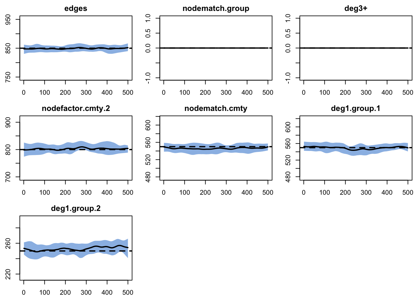
Finally, we run model diagnostics to ensure the fit is good.
A printing of the mydx object.
EpiModel Network Diagnostics
=======================
Diagnostic Method: Dynamic
Simulations: 25
Time Steps per Sim: 500

Formation Diagnostics
-----------------------
                  Target Sim Mean Pct Diff Sim SE Z Score
edges                850  848.854   -0.135  1.528  -0.750
nodematch.group        0    0.000      NaN    NaN     NaN
deg3+                  0    0.000      NaN    NaN     NaN
nodefactor.cmty.2    800  802.726    0.341  2.562   1.064
nodematch.cmty       550  546.068   -0.715  1.421  -2.767
deg1.group.1         550  549.459   -0.098  1.289  -0.420
deg1.group.2         250  252.933    1.173  0.914   3.210
                  SD(Sim Means) SD(Statistic)
edges                    11.437        19.618
nodematch.group           0.000         0.000
deg3+                     0.000         0.000
nodefactor.cmty.2        17.905        29.142
nodematch.cmty           10.468        17.587
deg1.group.1              8.247        17.322
deg1.group.2              5.909        13.832

Duration Diagnostics
-----------------------
      Target Sim Mean Pct Diff Sim SE Z Score SD(Sim Means)
edges    187   185.95   -0.562  0.664  -1.581             5
      SD(Statistic)
edges         6.803

Dissolution Diagnostics
-----------------------
      Target Sim Mean Pct Diff Sim SE Z Score SD(Sim Means)
edges  0.005    0.005   -0.091      0  -0.226             0
      SD(Statistic)
edges         0.003
Looks pretty good! We can also confirm with a plot:
If it is of interest, you can also extract the raw data that goes into producing these numerical summaries and plots.
   time sim edges nodematch.group deg3+ nodefactor.cmty.2
1     1   1   829               0     0               777
2     2   1   831               0     0               779
3     3   1   835               0     0               786
4     4   1   831               0     0               783
5     5   1   836               0     0               790
6     6   1   837               0     0               789
7     7   1   838               0     0               791
8     8   1   840               0     0               788
9     9   1   843               0     0               789
10   10   1   843               0     0               791
   nodematch.cmty deg1.group.1 deg1.group.2
1             522          559          257
2             524          561          253
3             525          567          247
4             520          569          247
5             522          574          242
6             524          575          241
7             527          580          240
8             528          578          234
9             528          575          237
10            526          573          235
47.6 Epidemic Simulation
To get the epidemic simulation started, we first need to parameterize the model with epidemic model parameters, initial conditions, and control settings (details provided here).
Code
myparam <- param.net(inf.prob = 0.6, inf.prob.g2 = 0.6,
                     act.rate = 1.8,
                     rec.rate = 0.1, rec.rate.g2 = 0.1)
myinit <- init.net(i.num = 100, i.num.g2 = 100)
mycontrol <- control.net("SIS", nsteps = 50, nsims = 5,
                         nwstats.formula = ~edges + nodematch("cmty") +
                         degree(0:5, by = "group"), verbose = TRUE)
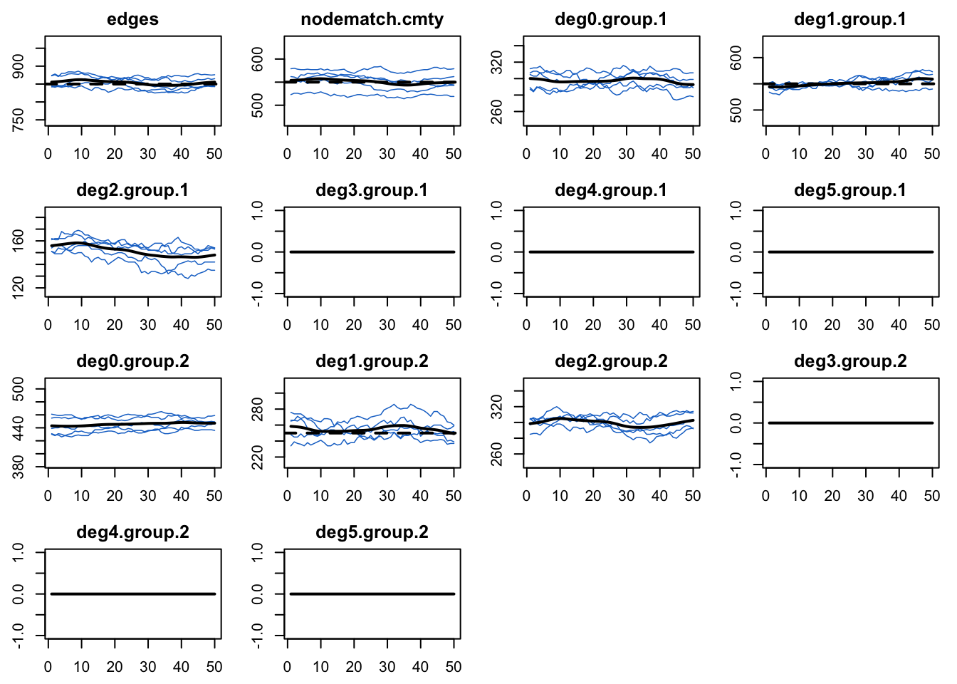
Note that we added in some additional degree terms for it to monitor, just to demonstrate that there are indeed no nodes with higher degrees.
Run the epidemic simulation with netsim.
Plot infection prevalence by group. Note that the prevalence in group 1 (females) is higher than group 2 (males). This would once again seem to be driven by the sex-specific differences in concurrency.
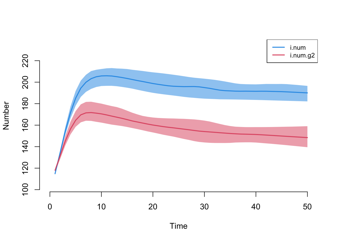
Here are numerical summaries for the sex-specific disease prevalence at the final time step.
Code
[1] 0.1906[1] 0.148We can also calculate and plot network stats as a time series from the epidemic simulations (to ensure that the epidemic simulations did not have unintended consequences on the network structure).