Epidemics with Multiple (Multilayer) Networks

multilayer networks

network structure

intermediate

Simulates epidemics on multilayer networks with shared nodes but distinct edge sets, modeling cross-layer dependency in partnership formation.

Author

Samuel M. Jenness

Published

December 1, 2022

Overview

This example demonstrates how to simulate an epidemic on a multilayer network in EpiModel. A multilayer network consists of two or more network layers that share the same node set but have different edge sets — representing distinct types of relationships. For example, the two layers might represent main partnerships and casual contacts, or sexual contacts and needle-sharing contacts.

The key feature of multilayer models is cross-layer dependency: the degree (number of edges) in one layer can influence edge formation in the other. This models the realistic constraint that individuals have finite relational capacity — being active in one type of partnership reduces availability for the other. The cross-layer dependency is maintained during simulation by a callback function that updates degree attributes between layer resimulations.

This example uses a simple SI model in a closed population to isolate the multilayer network mechanics from disease model complexity. No custom module-fx.R is needed — it uses EpiModel’s built-in SI modules. The multilayer functionality is entirely in the network estimation and simulation layers.

Download standalone script

model.R — Main simulation script (no module-fx.R needed for this example)

Model Structure

Compartment	Label	Description
Susceptible	S	Not infected; at risk of infection through contact on either network layer
Infectious	I	Infected and capable of transmitting (no recovery in SI)

flowchart LR
    S["<b>S</b><br/>Susceptible"] -->|"infection<br/>(si.flow)"| I["<b>I</b><br/>Infectious"]

    style S fill:#3498db,color:#fff
    style I fill:#e74c3c,color:#fff

Network Layers

The two network layers have different formation models, target statistics, and mean durations. Transmission can occur over edges in either layer.

Property	Layer 1	Layer 2
Interpretation	Longer-duration partnerships	Shorter-duration partnerships
Target edges	90	75
Mean degree	0.36	0.30
Mean duration	100 time steps	75 time steps
Formation terms	`edges + nodematch("race") + nodefactor("deg1+.net2")`	`edges + degree(1) + nodefactor("deg1+.net1")`
Cross-layer term	`nodefactor("deg1+.net2")`	`nodefactor("deg1+.net1")`

Cross-Layer Dependency

The nodefactor("deg1+.netX") terms create negative degree correlation across layers. The target statistic for these terms (10 out of 90 or 75 total edges) is deliberately small relative to total edges, producing strong negative correlation: most nodes that are active in one layer are inactive in the other.

Setup

suppressMessages(library(EpiModel))

nsims <- 5
ncores <- 5
nsteps <- 500

Network Model

Network Initialization

Initialize a network of 500 nodes with a binary demographic attribute (race). This attribute is used for assortative mixing (homophily) in layer 1’s formation model.

n <- 500
nw <- network_initialize(n)
nw <- set_vertex_attribute(nw, "race", rep(0:1, length.out = n))

Generating Starting Degree Values with `san()`

Because the two layers depend on each other’s degree distribution (via cross-layer nodefactor terms), we need reasonable starting values for the degree attributes before fitting the ERGM models. We use san() (simulated annealing from the ergm package) to generate edge sets consistent with our target statistics.

Step 1: Generate layer 1 edges consistent with target mean degree and race homophily. Layer 1 has target stats of 90 total edges and 60 that are race-homophilous (same-race partnerships).

nw_san <- san(nw ~ edges + nodematch("race"), target.stats = c(90, 60))

1nw_san <- set_vertex_attribute(nw_san, "deg.net1", get_degree(nw_san))
nw_san <- set_vertex_attribute(nw_san, "deg1+.net1",
2                               pmin(get_degree(nw_san), 1))

1: Record each node’s exact degree in layer 1 as a vertex attribute.
2: Create a binary indicator (0 vs. 1+) for the cross-layer formation term.

Step 2: Generate layer 2 edges, accounting for the cross-layer constraint from step 1. The nodefactor("deg1+.net1") term ensures that nodes already active in layer 1 are less likely to form layer 2 edges (negative correlation).

nw_san_2 <- san(nw_san ~ edges + degree(1) + nodefactor("deg1+.net1")
                  + Sum(matrix(seq_len(network.size(nw)), nrow = 1) ~
                        degrange(1, by = "deg.net1", levels = -1),
                    label = "Sum"),
1                target.stats = c(75, 120, 10, 10))
nw_san <- set_vertex_attribute(nw_san, "deg1+.net2",
                               pmin(get_degree(nw_san_2), 1))

1: Targets: 75 total edges, 120 degree-1 nodes, 10 edges involving nodes active in layer 1, and 10 for the Sum term linking layer 2 degree to layer 1 degree categories.

Verify that both SAN networks approximate their target statistics. These do not need to be exact — they are starting conditions for the ERGM estimation.

# Layer 1 targets: 90 edges, 60 homophilous
summary(nw_san ~ edges + nodematch("race") + nodefactor("deg1+.net2"))

                  edges          nodematch.race nodefactor.deg1+.net2.1 
                     90                      60                      10

# Layer 2 targets: 75 edges, 120 degree-1
summary(nw_san_2 ~ edges + degree(1) + nodefactor("deg1+.net1"))

                  edges                 degree1 nodefactor.deg1+.net1.1 
                     75                     120                      10

Set the binary degree attributes on the original network object for estimation.

nw <- set_vertex_attribute(nw, "deg1+.net1", pmin(get_degree(nw_san), 1))
nw <- set_vertex_attribute(nw, "deg1+.net2", pmin(get_degree(nw_san_2), 1))

Network Model Estimation

The formation models include both layer-specific terms and cross-layer dependency terms. Layer 1 models race homophily; layer 2 models the degree-1 count. Both include a nodefactor term for the other layer’s degree, creating negative degree correlation across layers.

formation.1 <- ~edges + nodematch("race") + nodefactor("deg1+.net2")
formation.2 <- ~edges + degree(1) + nodefactor("deg1+.net1")

1target.stats.1 <- c(90, 60, 10)
2target.stats.2 <- c(75, 120, 10)

1: Layer 1: 90 edges total, 60 race-homophilous, 10 among nodes with layer-2 edges (strong negative correlation).
2: Layer 2: 75 edges total, 120 degree-1 nodes, 10 among nodes with layer-1 edges.

Dissolution models specify the mean partnership duration for each layer independently.

1coef.diss.1 <- dissolution_coefs(dissolution = ~offset(edges), duration = 100)
2coef.diss.2 <- dissolution_coefs(dissolution = ~offset(edges), duration = 75)

1: Layer 1: longer, more stable partnerships (mean duration 100 time steps).
2: Layer 2: shorter, more transient partnerships (mean duration 75 time steps).

Although we think of this as one multilayer network, estimation is done separately for each layer. The layers are linked through the shared nodal attributes (deg1+.net1, deg1+.net2).

est.1 <- netest(nw, formation.1, target.stats.1, coef.diss.1)
est.2 <- netest(nw, formation.2, target.stats.2, coef.diss.2)

Network Diagnostics

Run diagnostics for each layer. Because the network is relatively small (500 nodes) and some target statistics are small (10 for cross-layer terms), there may be more variability than in a single-layer model.

dx.1 <- netdx(est.1, nsims = nsims, ncores = ncores, nsteps = nsteps)


Network Diagnostics
-----------------------
- Simulating 5 networks
- Calculating formation statistics

print(dx.1)

EpiModel Network Diagnostics
=======================
Diagnostic Method: Dynamic
Simulations: 5
Time Steps per Sim: 500

Formation Diagnostics
----------------------- 
                        Target Sim Mean Pct Diff Sim SE Z Score SD(Sim Means)
edges                       90   88.612   -1.542  1.032  -1.344         3.101
nodematch.race              60   60.950    1.583  0.991   0.958         4.306
nodefactor.deg1+.net2.1     10   10.928    9.280  0.603   1.540         2.323
                        SD(Statistic)
edges                           6.793
nodematch.race                  6.476
nodefactor.deg1+.net2.1         3.362

Duration Diagnostics
----------------------- 
      Target Sim Mean Pct Diff Sim SE Z Score SD(Sim Means) SD(Statistic)
edges    100   98.604   -1.396  1.742  -0.801         5.678         9.827

Dissolution Diagnostics
----------------------- 
      Target Sim Mean Pct Diff Sim SE Z Score SD(Sim Means) SD(Statistic)
edges   0.01     0.01   -3.571      0  -1.734             0          0.01

plot(dx.1)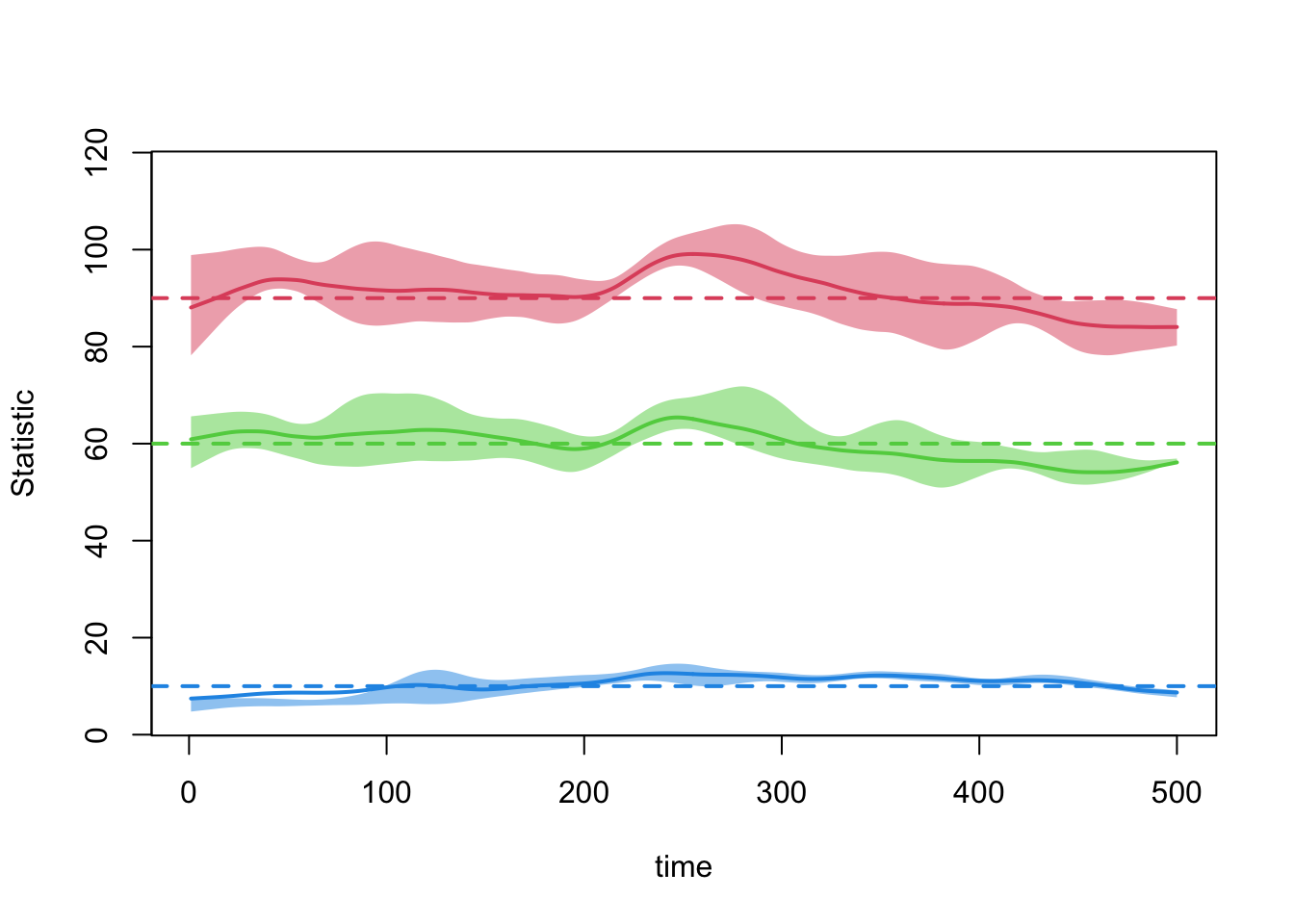

Figure 1: Layer 1 network diagnostics verifying formation statistics track their targets.

dx.2 <- netdx(est.2, nsims = nsims, ncores = ncores, nsteps = nsteps)


Network Diagnostics
-----------------------
- Simulating 5 networks
- Calculating formation statistics

print(dx.2)

EpiModel Network Diagnostics
=======================
Diagnostic Method: Dynamic
Simulations: 5
Time Steps per Sim: 500

Formation Diagnostics
----------------------- 
                        Target Sim Mean Pct Diff Sim SE Z Score SD(Sim Means)
edges                       75   76.048    1.398  1.108   0.946         1.788
degree1                    120  118.266   -1.445  1.547  -1.121         2.777
nodefactor.deg1+.net1.1     10   11.005   10.052  0.622   1.616         1.685
                        SD(Statistic)
edges                           6.953
degree1                        10.080
nodefactor.deg1+.net1.1         3.218

Duration Diagnostics
----------------------- 
      Target Sim Mean Pct Diff Sim SE Z Score SD(Sim Means) SD(Statistic)
edges     75   78.181    4.242  1.535   2.073         3.463         8.179

Dissolution Diagnostics
----------------------- 
      Target Sim Mean Pct Diff Sim SE Z Score SD(Sim Means) SD(Statistic)
edges  0.013    0.013    -0.54      0  -0.256             0         0.013

plot(dx.2)

Figure 2: Layer 2 network diagnostics verifying formation statistics track their targets.

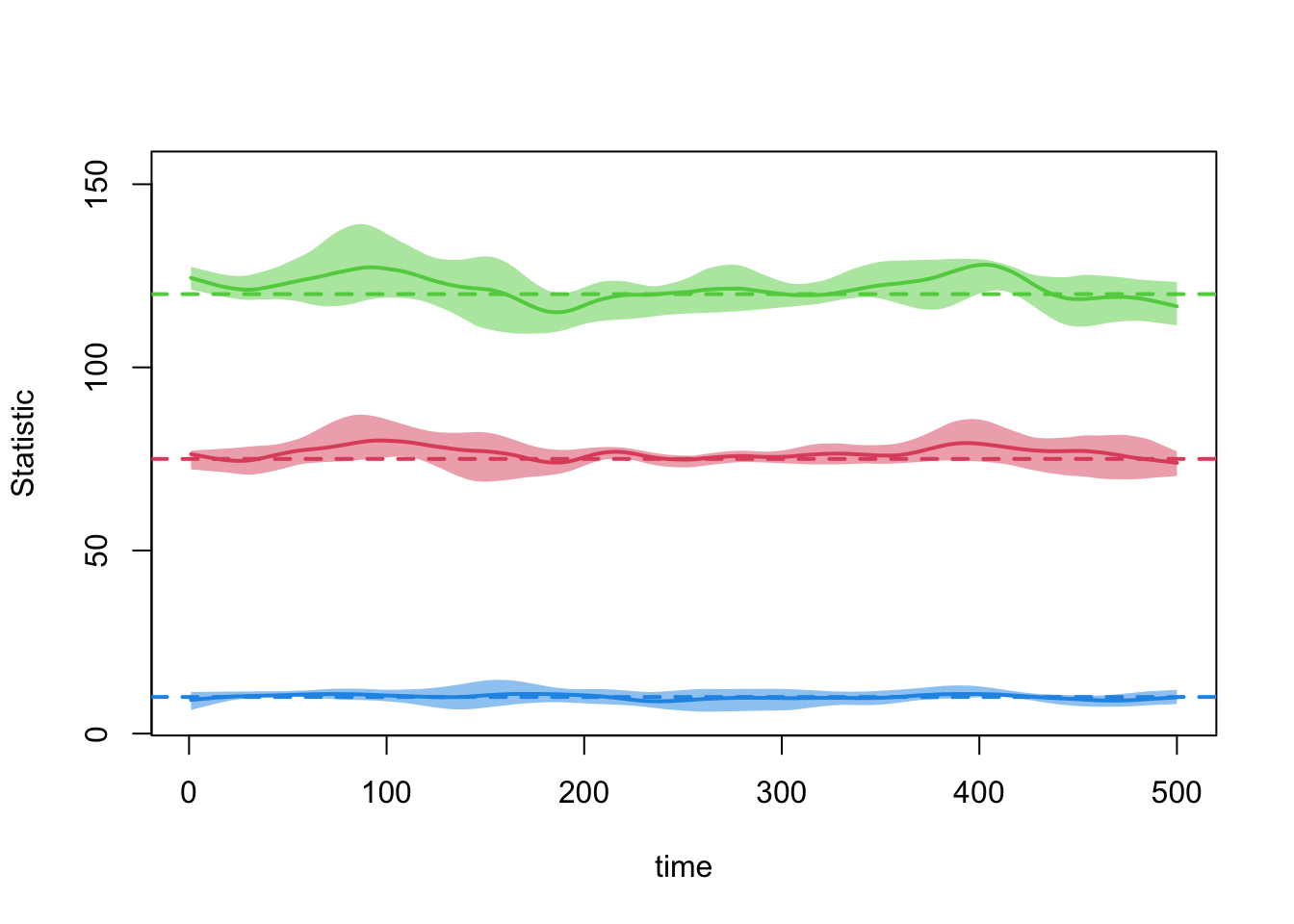
Epidemic Simulation

Parameters

Simple SI model parameters. The high transmission probability and act rate are deliberate — they generate a clearly visible epidemic so we can focus on the network mechanics rather than epidemiological realism.

1param <- param.net(inf.prob = 0.5, act.rate = 2)
2init <- init.net(i.num = 10)

1: Per-act transmission probability of 0.5 with 2 acts per partnership per time step.
2: Start with 10 infected individuals (2% initial prevalence in 500 nodes).

Cross-Layer Update Function

This is the key mechanism for multilayer feedback. During each time step, EpiModel resimulates each network layer sequentially. Before resimulating layer k, it calls this function to update the cross-layer degree attributes that layer k’s formation model depends on. Without this function, the cross-layer degree attributes would be frozen at their initial values and the layers would evolve independently.

network_layer_updates <- function(dat, at, network) {
  if (network == 0) {
1    dat <- set_attr(dat, "deg1+.net2", pmin(get_degree(dat$run$el[[2]]), 1))
  } else if (network == 1) {
2    dat <- set_attr(dat, "deg1+.net1", pmin(get_degree(dat$run$el[[1]]), 1))
  } else if (network == 2) {
3    dat <- set_attr(dat, "deg1+.net2", pmin(get_degree(dat$run$el[[2]]), 1))
  }
  return(dat)
}

1: network == 0 (before layer 1 resimulation): update deg1+.net2 from current layer 2 edges.
2: network == 1 (before layer 2 resimulation): update deg1+.net1 from current layer 1 edges.
3: network == 2 (after layer 2 resimulation): recalculate deg1+.net2 for summary statistics.

Control Settings and Simulation

control <- control.net(
  type = "SI",
  nsteps = nsteps,
  nsims = nsims,
  ncores = ncores,
1  tergmLite = TRUE,
2  resimulate.network = TRUE,
3  dat.updates = network_layer_updates,
4  nwstats.formula = multilayer(
    "formation",
    ~edges + nodefactor("deg1+.net1") + degree(0:4)
  )
)

5sim <- netsim(list(est.1, est.2), param, init, control)

1: Use lightweight edgelist representation (required for dat$run$el[[]] access in the update callback).
2: Redraw both layers each time step.
3: The cross-layer degree update callback runs between layer resimulations.
4: multilayer() specifies per-layer network statistics to track. Layer 1 uses the default formation formula; layer 2 additionally tracks the full degree distribution (degree 0 through 4).
5: Passing a list of netest objects tells EpiModel this is a multilayer model. The list order determines layer numbering.

Analysis

Network Formation During Simulation

Verify that network structure is maintained during the epidemic. These plots should show the simulated formation statistics tracking close to their targets throughout the run.

par(mfrow = c(1, 1), mar = c(3, 3, 2, 1), mgp = c(2, 1, 0))
print(sim, network = 1)

EpiModel Simulation
=======================
Model class: netsim

Simulation Summary
-----------------------
Model type: SI
No. simulations: 5
No. time steps: 500
No. NW groups: 1

Fixed Parameters
---------------------------
inf.prob = 0.5
act.rate = 2
groups = 1

Model Output
-----------------------
Variables: s.num i.num num si.flow
Networks: sim1 ... sim5
Transmissions: sim1 ... sim5

Formation Statistics
----------------------- 
                        Target Sim Mean Pct Diff Sim SE Z Score SD(Sim Means)
edges                       90   95.111    5.679  2.446   2.090         7.621
nodematch.race              60   63.020    5.033  1.757   1.719         2.938
nodefactor.deg1+.net2.1     10   12.030   20.300  0.799   2.541         2.211
                        SD(Statistic)
edges                          11.476
nodematch.race                  8.344
nodefactor.deg1+.net2.1         4.510


Duration and Dissolution Statistics
----------------------- 
Not available when:
- `control$tergmLite == TRUE`
- `control$save.network == FALSE`
- `control$save.diss.stats == FALSE`
- dissolution formula is not `~ offset(edges)`
- `keep.diss.stats == FALSE` (if merging)

plot(sim, network = 1, type = "formation",
     main = "Layer 1: Formation Diagnostics During Simulation")

Figure 3: Layer 1 formation diagnostics during the epidemic simulation.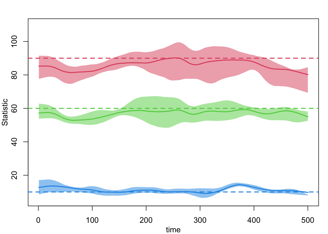

print(sim, network = 2)

EpiModel Simulation
=======================
Model class: netsim

Simulation Summary
-----------------------
Model type: SI
No. simulations: 5
No. time steps: 500
No. NW groups: 1

Fixed Parameters
---------------------------
inf.prob = 0.5
act.rate = 2
groups = 1

Model Output
-----------------------
Variables: s.num i.num num si.flow
Networks: sim1 ... sim5
Transmissions: sim1 ... sim5

Formation Statistics
----------------------- 
                        Target Sim Mean Pct Diff Sim SE Z Score SD(Sim Means)
edges                       75   69.847   -6.871  1.204  -4.280         3.461
nodefactor.deg1+.net1.1     10   11.085   10.848  0.832   1.304         1.764
degree0                     NA  374.315       NA  1.914      NA         6.030
degree1                    120  112.976   -5.853  1.614  -4.353         5.333
degree2                     NA   11.480       NA  0.457      NA         0.745
degree3                     NA    1.166       NA  0.142      NA         0.154
degree4                     NA    0.055       NA  0.010      NA         0.063
                        SD(Statistic)
edges                           7.129
nodefactor.deg1+.net1.1         4.390
degree0                        11.923
degree1                        10.693
degree2                         3.285
degree3                         1.038
degree4                         0.229


Duration and Dissolution Statistics
----------------------- 
Not available when:
- `control$tergmLite == TRUE`
- `control$save.network == FALSE`
- `control$save.diss.stats == FALSE`
- dissolution formula is not `~ offset(edges)`
- `keep.diss.stats == FALSE` (if merging)

plot(sim, network = 2, type = "formation",
     main = "Layer 2: Formation Diagnostics During Simulation")

Figure 4: Layer 2 formation diagnostics during the epidemic simulation.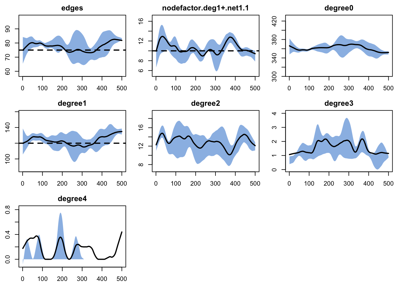

SI Compartment Counts

plot(sim, y = c("s.num", "i.num"),
     main = "SI Epidemic on Multilayer Network",
     ylab = "Count", xlab = "Time Steps",
     mean.col = c("steelblue", "firebrick"),
     mean.lwd = 2, mean.smooth = TRUE,
     qnts.col = c("steelblue", "firebrick"),
     qnts.alpha = 0.2, qnts.smooth = TRUE,
     legend = TRUE)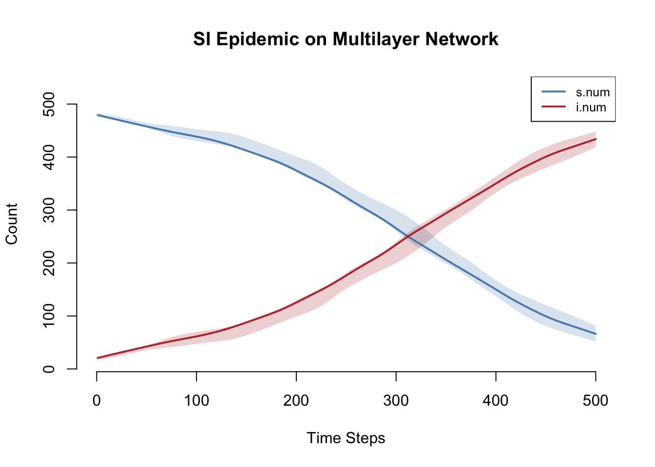

Figure 5: Susceptible and infected counts over time on the multilayer network.

Prevalence

sim <- mutate_epi(sim, prev = i.num / num)
plot(sim, y = "prev",
     main = "Prevalence over Time",
     ylab = "Prevalence", xlab = "Time Steps",
     mean.col = "firebrick", mean.lwd = 2, mean.smooth = TRUE,
     qnts.col = "firebrick", qnts.alpha = 0.2, qnts.smooth = TRUE)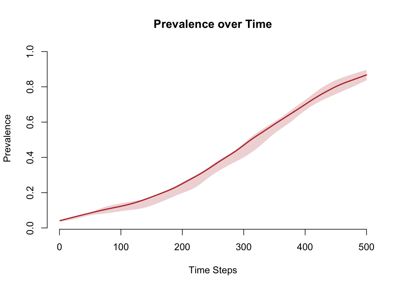

Incidence

plot(sim, y = "si.flow",
     main = "New Infections per Time Step",
     ylab = "Incidence", xlab = "Time Steps",
     mean.col = "firebrick", mean.lwd = 2, mean.smooth = TRUE,
     qnts.col = "firebrick", qnts.alpha = 0.2, qnts.smooth = TRUE)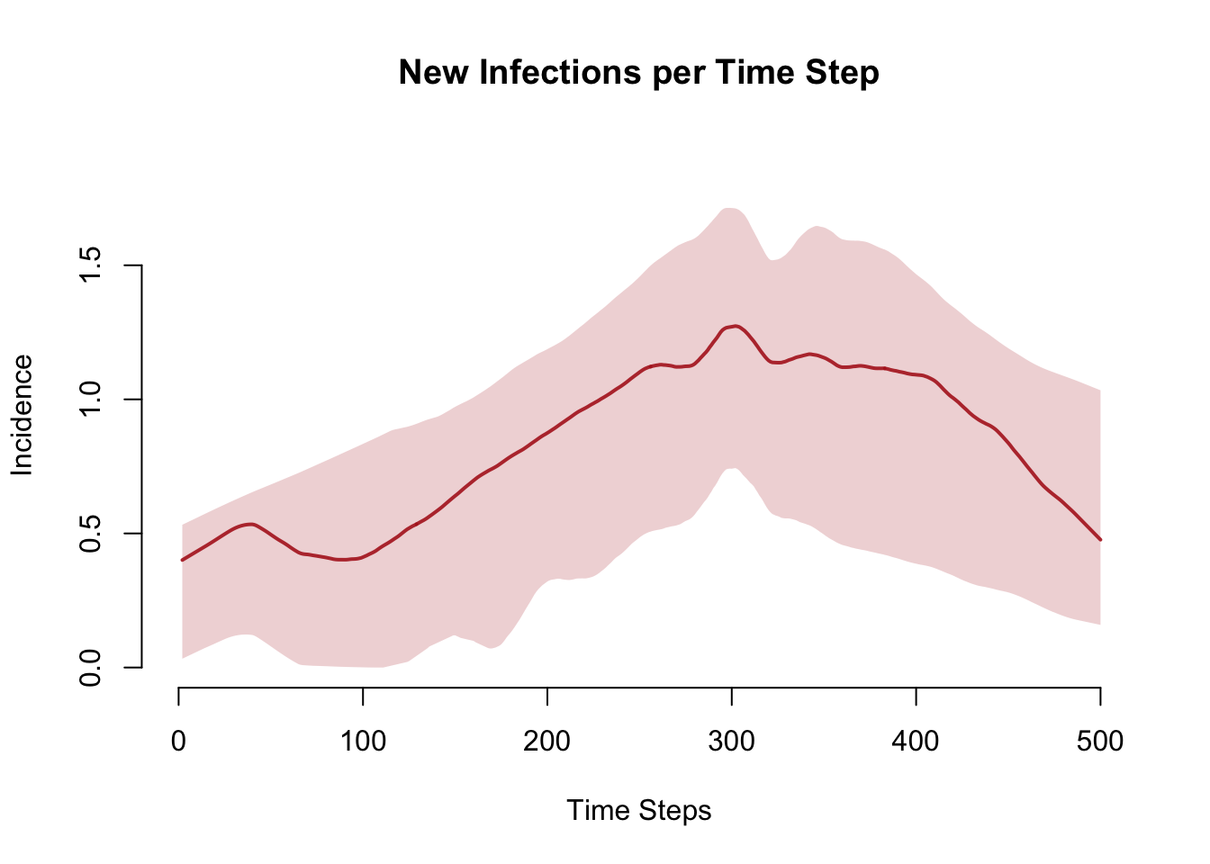

Summary Table

df <- as.data.frame(sim)
last_t <- max(df$time)

knitr::kable(data.frame(
  Metric = c("Population size",
             "Final susceptible",
             "Final infected",
             "Final prevalence",
             "Cumulative new infections",
             "Peak incidence (per time step)"),
  Value = c(n,
            round(mean(df$s.num[df$time == last_t])),
            round(mean(df$i.num[df$time == last_t])),
            round(mean(df$prev[df$time == last_t]), 3),
            round(mean(tapply(df$si.flow, df$sim, sum, na.rm = TRUE))),
            max(df$si.flow, na.rm = TRUE))
))

Table 1

Metric	Value
Population size	500.000
Final susceptible	63.000
Final infected	437.000
Final prevalence	0.874
Cumulative new infections	427.000
Peak incidence (per time step)	9.000

Parameters

Epidemic

Parameter	Description	Value
`inf.prob`	Per-act transmission probability	0.5
`act.rate`	Acts per partnership per time step	2

Network Formation

Parameter	Layer 1	Layer 2
Target edges	90	75
Race homophily (`nodematch`)	60	—
Degree-1 count (`degree(1)`)	—	120
Cross-layer `nodefactor`	10	10

Network Dissolution

Parameter	Layer 1	Layer 2
Mean duration (time steps)	100	75

Key EpiModel Functions for Multilayer Models

Function / Argument	Purpose
`netsim(list(est.1, est.2), ...)`	Passing a list of `netest` objects signals a multilayer model
`dat.updates` in `control.net()`	Callback function for cross-layer attribute updates
`multilayer()` in `nwstats.formula`	Specifies per-layer network statistics to track
`tergmLite = TRUE`	Uses lightweight edgelist representation (required for `dat$run$el[[]]` access)
`resimulate.network = TRUE`	Required for multilayer models with cross-layer dependency

Next Steps

Layer-specific transmission: different inf.prob or act.rate by edge type (e.g., lower transmission in casual vs. main partnerships)
More than two layers: add a third network layer (e.g., needle-sharing)
Vital dynamics: add arrivals and departures with custom modules — see SI with Vital Dynamics for the departure and arrival module pattern
Different disease models: extend to SIR, SEIR, or disease-specific models — see Adding an Exposed State for the progression module pattern
Heterogeneous populations: add more nodal attributes beyond the binary race attribute used here

Overview

Model Structure

Network Layers

Cross-Layer Dependency

Setup

Network Model

Network Initialization

Generating Starting Degree Values with san()

Network Model Estimation

Network Diagnostics

Epidemic Simulation

Parameters

Cross-Layer Update Function

Control Settings and Simulation

Analysis

Network Formation During Simulation

SI Compartment Counts

Prevalence

Incidence

Summary Table

Parameters

Epidemic

Network Formation

Network Dissolution

Key EpiModel Functions for Multilayer Models

Next Steps

Generating Starting Degree Values with `san()`