flowchart LR
    S["<b>S</b><br/>Susceptible"] -->|"infection<br/>(si.flow)"| I["<b>I</b><br/>Infectious"]
    style S fill:#3498db,color:#fff
    style I fill:#e74c3c,color:#fff
Multilayer Networks: Independent Layers
SI
multilayer networks
network structure
beginner
The simplest multilayer model: an SI epidemic over two independent network layers (same nodes, different edge sets). The entry point to multilayer modeling, before cross-layer dependency.
Overview
A multilayer network is two or more network layers that share the same node set but have different edge sets, representing distinct kinds of relationships. For example, the same people may have main partnerships (steady, long-lasting) and casual partnerships (more transient). An epidemic can spread over edges in either layer.
This example is the entry point to multilayer modeling. The two layers here are independent: a person’s number of partners in one layer does not constrain the other. That keeps the mechanics minimal, so the only genuinely new idea is that you fit each layer as an ordinary network model and then hand netsim() a list of them. There is no simulated annealing, no cross-layer attribute, and no update callback. Those are needed only when the layers depend on each other, which is the companion Multilayer Networks (cross-layer dependency) example.
If you have built a single-layer network model before (an edges model with netest() and netsim()), you already know almost everything here.
TipDownload standalone script
- model.R — Main simulation script (no
module-fx.Rneeded; built-in SI modules)
Model Structure
| Compartment | Label | Description |
|---|---|---|
| Susceptible | S | Not infected; at risk via contact on either layer |
| Infectious | I | Infected and capable of transmitting (no recovery in SI) |
The key picture to hold in mind: one set of people, two separate edge sets drawn over them. A node can have several main partners and no casual partners, or the reverse. Because the layers are independent here, those two partner counts are unrelated.
| Property | Layer 1 (main) | Layer 2 (casual) |
|---|---|---|
| Interpretation | Steady, long-lasting partnerships | Transient, higher-turnover contacts |
| Target edges | 90 | 75 |
| Formation terms | edges + nodematch("race") |
edges + degree(1) |
| Mean duration | 200 time steps | 20 time steps |
| Cross-layer term | none (independent) | none (independent) |
Setup
suppressMessages(library(EpiModel))

nsims <- 5
ncores <- 5
nsteps <- 500
Network Model
One shared node set carries both layers. We add a binary race attribute used for homophily in layer 1.
n <- 500
nw <- network_initialize(n)
nw <- set_vertex_attribute(nw, "race", rep(0:1, length.out = n))
Each layer is an ordinary single-layer TERGM, fit exactly as in the earlier Gallery examples. Nothing here is multilayer-specific yet.
- 1
- Layer 1: 90 edges total (mean degree 0.36), 60 of them race-homophilous.
- 2
- Layer 1 ties are long-lasting (mean duration 200 time steps).
- 3
-
Layer 2’s formation references only its own structure (
degree(1)); it does not reference layer 1. That independence is what removes the need for any cross-layer machinery. - 4
- Layer 2 ties turn over quickly (mean duration 20 time steps), the main-vs-casual contrast.
Diagnostics
Diagnose each layer separately, as you would any single-layer model.
dx1 <- netdx(est1, nsims = nsims, ncores = ncores, nsteps = nsteps)
Network Diagnostics
-----------------------
- Simulating 5 networks
- Calculating formation statisticsprint(dx1)EpiModel Network Diagnostics
=======================
Diagnostic Method: Dynamic
Simulations: 5
Time Steps per Sim: 500
Formation Diagnostics
-----------------------
Target Sim Mean Pct Diff Sim SE Z Score SD(Sim Means)
edges 90 87.658 -2.602 1.449 -1.616 6.651
nodematch.race 60 59.190 -1.351 1.209 -0.670 3.877
SD(Statistic)
edges 8.058
nodematch.race 5.910
Duration Diagnostics
-----------------------
Target Sim Mean Pct Diff Sim SE Z Score SD(Sim Means) SD(Statistic)
edges 200 203.373 1.686 4.032 0.837 12.322 19.226
Dissolution Diagnostics
-----------------------
Target Sim Mean Pct Diff Sim SE Z Score SD(Sim Means) SD(Statistic)
edges 0.005 0.005 1.094 0 0.365 0 0.008plot(dx1)
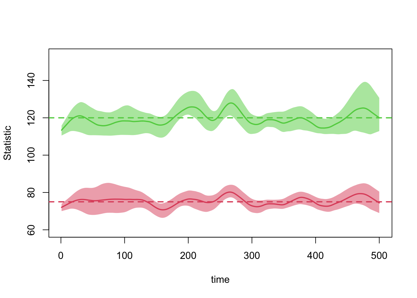
dx2 <- netdx(est2, nsims = nsims, ncores = ncores, nsteps = nsteps)
Network Diagnostics
-----------------------
- Simulating 5 networks
- Calculating formation statisticsprint(dx2)EpiModel Network Diagnostics
=======================
Diagnostic Method: Dynamic
Simulations: 5
Time Steps per Sim: 500
Formation Diagnostics
-----------------------
Target Sim Mean Pct Diff Sim SE Z Score SD(Sim Means) SD(Statistic)
edges 75 75.434 0.578 0.874 0.496 1.899 8.295
degree1 120 119.623 -0.314 1.190 -0.317 2.926 12.398
Duration Diagnostics
-----------------------
Target Sim Mean Pct Diff Sim SE Z Score SD(Sim Means) SD(Statistic)
edges 20 19.749 -1.253 0.203 -1.234 0.461 2.039
Dissolution Diagnostics
-----------------------
Target Sim Mean Pct Diff Sim SE Z Score SD(Sim Means) SD(Statistic)
edges 0.05 0.05 -0.759 0.001 -0.685 0.001 0.026plot(dx2)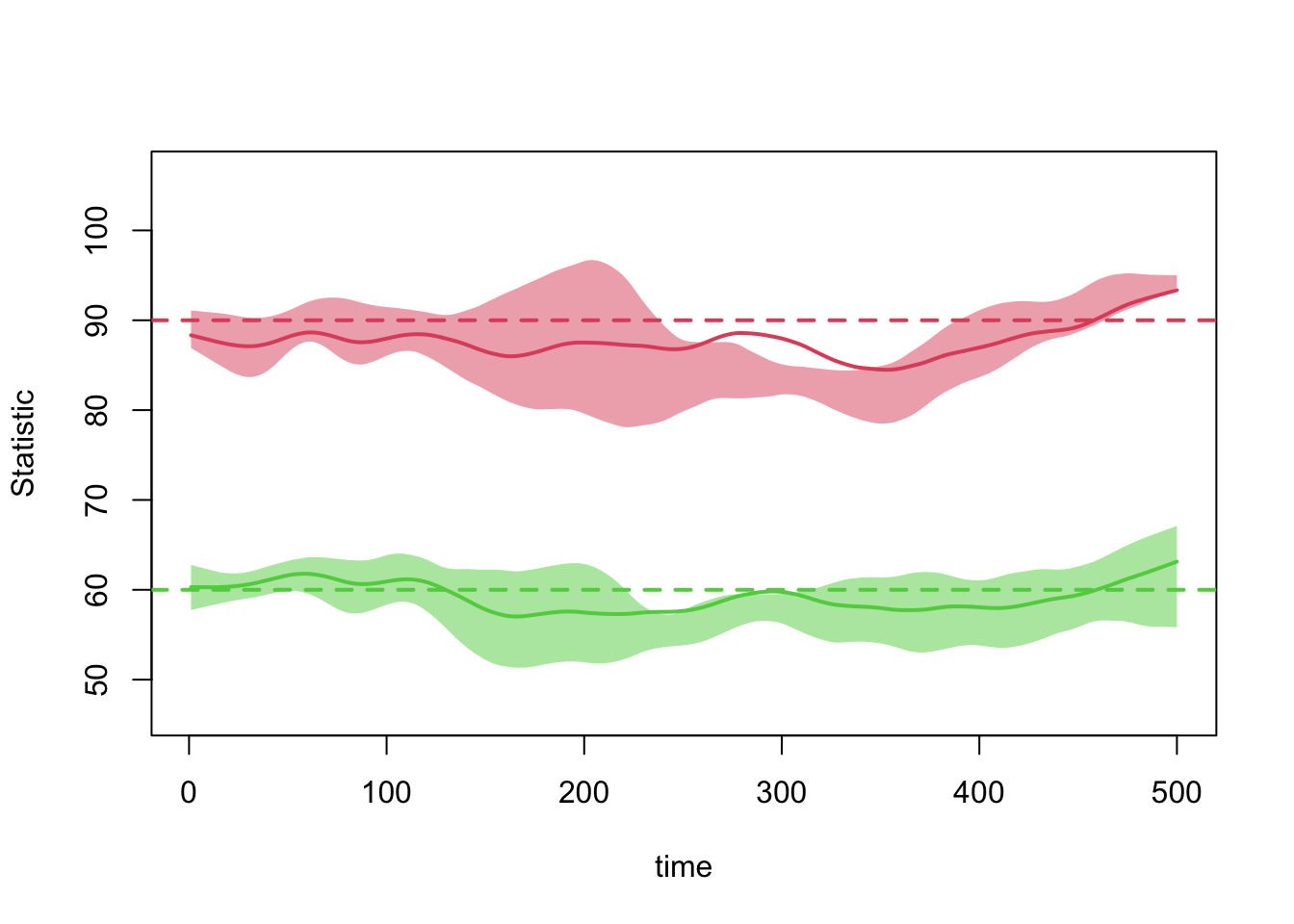
Epidemic Simulation
A simple SI model in a closed population, so the focus stays on the network mechanics. Transmission can occur over edges in either layer.
param <- param.net(inf.prob = 0.5, act.rate = 2)
init <- init.net(i.num = 10)
The control settings differ from a single-layer model in only two ways, and one of them is optional.
- 1
- Redraw both layers each time step. Required whenever the network is dynamic.
- 2
-
multilayer()maps a per-layer diagnostic formula to each layer by position. This is optional; omit it and EpiModel tracks each layer’s own formation formula by default. - 3
-
Passing a list of
netestobjects is the one step that makes this multilayer. The list order is the layer numbering. Note what is absent: nosan(), no cross-layer attributes, and nodat.updatescallback are needed, because neither layer’s formation model reads from the other.
Analysis
First confirm the network structure held up during the run.
print(sim, network = 1)EpiModel Simulation
=======================
Model class: netsim
Simulation Summary
-----------------------
Model type: SI
No. simulations: 5
No. time steps: 500
No. NW groups: 1
Fixed Parameters
---------------------------
inf.prob = 0.5
act.rate = 2
groups = 1
Model Output
-----------------------
Variables: s.num i.num num si.flow
Networks: sim1 ... sim5
Transmissions: sim1 ... sim5
Formation Statistics
-----------------------
Target Sim Mean Pct Diff Sim SE Z Score SD(Sim Means)
edges 90 95.142 5.713 2.236 2.300 9.702
nodematch.race 60 61.643 2.739 2.214 0.742 8.798
SD(Statistic)
edges 11.007
nodematch.race 9.961
Duration and Dissolution Statistics
-----------------------
Not available when:
- `control$tergmLite == TRUE`
- `control$save.network == FALSE`
- `control$save.diss.stats == FALSE`
- dissolution formula is not `~ offset(edges)`
- `keep.diss.stats == FALSE` (if merging)plot(sim, network = 1, type = "formation", main = "Layer 1 (main) formation")
print(sim, network = 2)EpiModel Simulation
=======================
Model class: netsim
Simulation Summary
-----------------------
Model type: SI
No. simulations: 5
No. time steps: 500
No. NW groups: 1
Fixed Parameters
---------------------------
inf.prob = 0.5
act.rate = 2
groups = 1
Model Output
-----------------------
Variables: s.num i.num num si.flow
Networks: sim1 ... sim5
Transmissions: sim1 ... sim5
Formation Statistics
-----------------------
Target Sim Mean Pct Diff Sim SE Z Score SD(Sim Means) SD(Statistic)
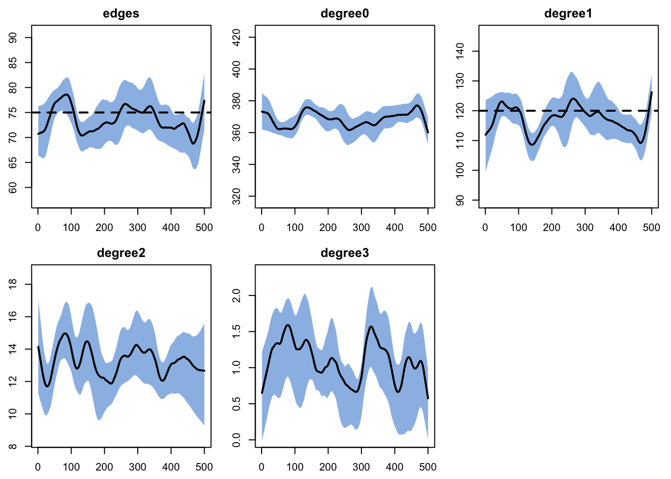
edges 75 73.539 -1.948 0.882 -1.656 0.719 7.982
degree0 NA 368.604 NA 1.477 NA 1.453 13.477
degree1 120 116.982 -2.515 1.279 -2.359 1.463 12.310
degree2 NA 13.230 NA 0.299 NA 0.384 3.766
degree3 NA 1.105 NA 0.073 NA 0.132 1.076
Duration and Dissolution Statistics
-----------------------
Not available when:
- `control$tergmLite == TRUE`
- `control$save.network == FALSE`
- `control$save.diss.stats == FALSE`
- dissolution formula is not `~ offset(edges)`
- `keep.diss.stats == FALSE` (if merging)plot(sim, network = 2, type = "formation", main = "Layer 2 (casual) formation")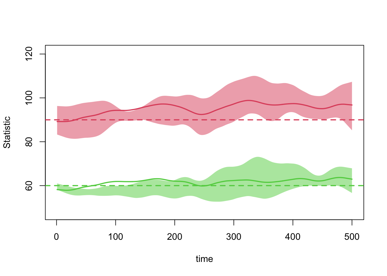
Now the epidemiological payoff: the disease curve over the two-layer network.
par(mfrow = c(1, 1), mar = c(3, 3, 2, 1), mgp = c(2, 1, 0))
plot(sim, y = c("s.num", "i.num"), legend = TRUE,
main = "SI Epidemic on Two Independent Layers")
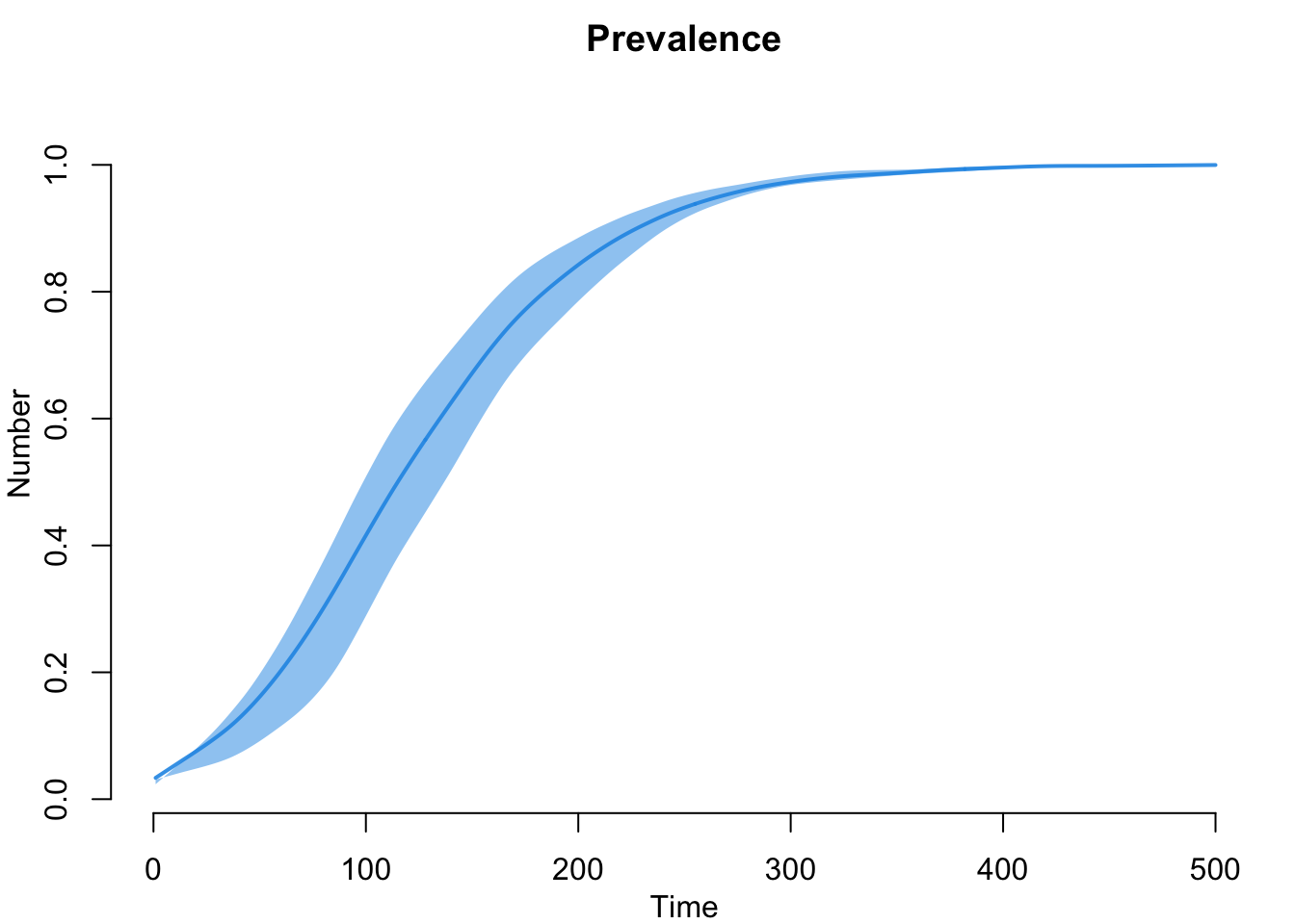
sim <- mutate_epi(sim, prev = i.num / num)
plot(sim, y = "prev", main = "Prevalence", legend = FALSE)
plot(sim, y = "si.flow", main = "Incidence (new infections per step)", legend = FALSE)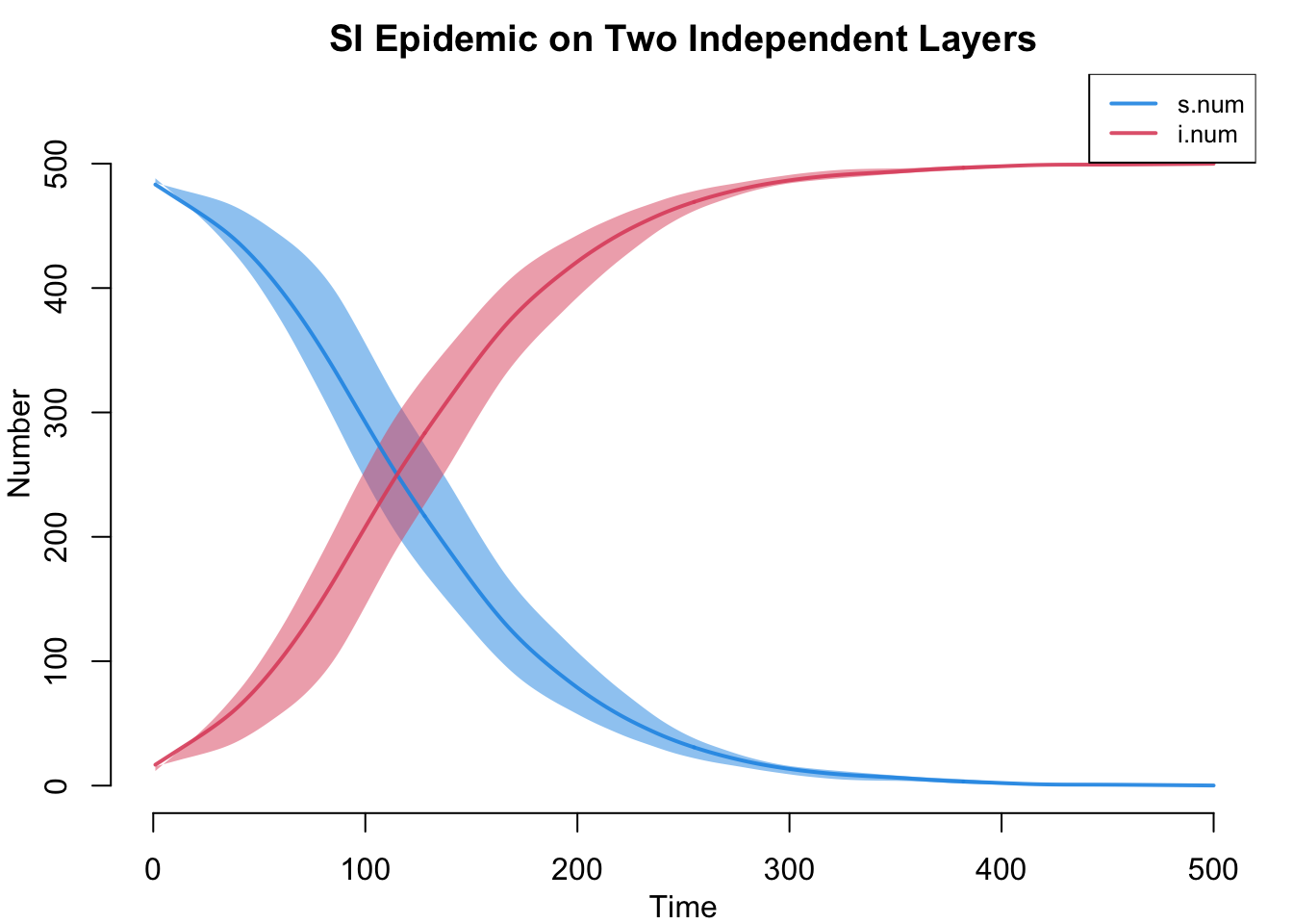
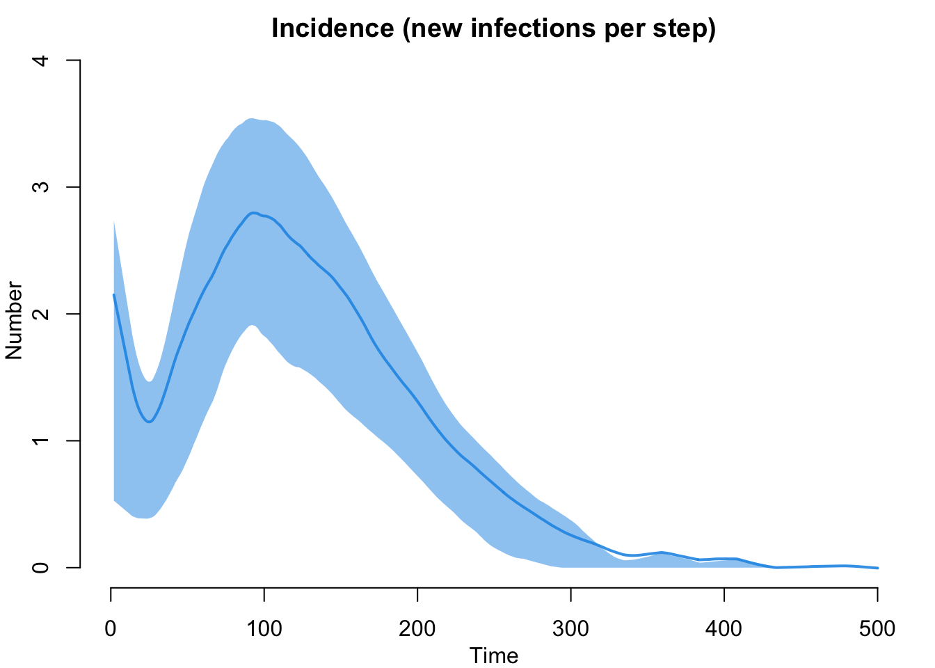
The short-duration casual layer tends to drive early spread, while the long-duration main layer sustains transmission over time. Because transmission can occur on either layer, the overall epidemic reflects contributions from both.
Parameters
| Parameter | Description | Value |
|---|---|---|
inf.prob |
Per-act transmission probability | 0.5 |
act.rate |
Acts per partnership per time step | 2 |
| Layer 1 edges / homophily | edges / nodematch("race") |
90 / 60 |
| Layer 2 edges / degree-1 | edges / degree(1) |
75 / 120 |
| Layer 1 / Layer 2 duration | mean edge duration | 200 / 20 |
Key EpiModel Functions for Multilayer Models
| Function / Argument | Purpose |
|---|---|
netsim(list(est1, est2), ...) |
Passing a list of netest objects signals a multilayer model; list order sets layer numbering |
resimulate.network = TRUE |
Redraw the dynamic layers each time step |
multilayer() in nwstats.formula |
Optional per-layer diagnostic statistics |
print(sim, network = k) / plot(sim, network = k, ...) |
Inspect a specific layer |
Next Steps
- Cross-layer dependency: make a person’s activity in one layer reduce their activity in the other (finite relational capacity, negative degree correlation). This adds a cross-layer formation term, a one-time
san()bootstrap, and an update callback. See Multilayer Networks (cross-layer dependency). - Layer-specific transmission: different
inf.proboract.rateby edge type (e.g., lower transmission on casual ties). - More than two layers: add a third layer (e.g., a one-off contact layer with
duration = 1) and passnetsim(list(est1, est2, est3), ...). - Different disease models: extend to SIR or SEIR using a custom progression module, see Adding an Exposed State.