30 Dynamic Network Visualization
This tutorial demonstrates methods for dynamic visualization of the spread of infectious disease over networks using the ndtv package for R. ndtv is part of the larger Statnet suite of software for the representation, modeling, and analysis of network data. It has been designed to work with network-based epidemic modeling data from EpiModel.
Download the R script to follow along with this tutorial here.
30.1 Setup
We start by loading EpiModel and ndtv. The htmlwidgets library additionally allows for embedding ndtv movies into RMarkdown HTML pages like this (you do not need to install/load it for this course but we need it to build this page).
In general, one primary goal of dynamic network visualization is to gain insight into how the structure of networks over time can influence transmission dynamics. This is different from estimating epidemic outcomes such as disease incidence or prevalence over time. The latter will typically require large networks (thousands of nodes) over large numbers of time steps (decades of time) with many hundreds or thousands of simulations. This allows for more accurate and stable estimation of outcome averages and spread. Dynamic visualization, on the other hand, usually only requires a single simulation of a small network size over a short number of time steps. That is because the visualization is meant to demonstrate the mechanisms rather than estimate the effects.
30.2 Model 1: Edges-Only
We start by setting a seed to ensure reproducible results. You can skip this to get different results from the tutorial page.
30.2.1 Epidemic Model
This shows an SI epidemic in a closed population where the infection probability is 1, and we will start to build up complexity to the network model step-by-step. We start with a network of 100 nodes, with an edges-only model in the formation and dissolution.
For the epidemic model, we will replicate the poker chip example in which the transmission probability per act is 100%. We could modify this to be a lower (more relistic for most diseases) value, but we choose a high value here to show a speedy epidemic spread. We simulate the model over 25 time steps with a single simulation.
30.2.2 Network Visualization
ndtv is an extension package in Statnet that allows for dynamic visualization for networks over time. Because this involves animation processing, this may require some heavy duty computation.
30.2.2.1 Extract and Process the Networks
First we need to extract the network objects from the larger netsim object. This was one of the key uses of this object type first discussed in Session 3 today. Note that this object has details on the distinct time changes.
NetworkDynamic properties:
distinct change times: 27
maximal time range: 0 until Inf
Dynamic (TEA) attributes:
Vertex TEAs: testatus.active
Includes optional net.obs.period attribute:
Network observation period info:
Number of observation spells: 2
Maximal time range observed: 0 until 26
Temporal mode: discrete
Time unit: step
Suggested time increment: 1
Network attributes:
vertices = 100
directed = FALSE
hyper = FALSE
loops = FALSE
multiple = FALSE
bipartite = FALSE
net.obs.period: (not shown)
vertex.pid = tergm_pid
total edges= 104
missing edges= 0
non-missing edges= 104
Vertex attribute names:
active status tergm_pid testatus.active vertex.names
Edge attribute names:
active Next, we need to add a time-varying nodal attribute to each network that we will animate. This will allow ndtv to color the nodes by disease status over time. See the help documentation for color_tea to see some of the options and details for this step.
30.2.2.2 Revisiting Static Visualizations
Before we start making a movie with this updated network object, recall the types of static visualizations of the co-evolving dynamic network and epidemic data that are possible with EpiModel. One approach is to extract and work with the transmission matrix within the netsim object.
# A tibble: 39 × 8
# Groups: at, sus [39]
at sus inf network infDur transProb actRate finalProb
<dbl> <int> <int> <int> <dbl> <dbl> <dbl> <dbl>
1 2 13 64 1 16 1 1 1
2 2 47 64 1 16 1 1 1
3 3 72 47 1 1 1 1 1
4 4 67 64 1 18 1 1 1
5 8 81 67 1 4 1 1 1
6 9 1 81 1 1 1 1 1
7 10 29 67 1 6 1 1 1
8 10 68 1 1 1 1 1 1
9 11 16 68 1 1 1 1 1
10 11 57 68 1 1 1 1 1
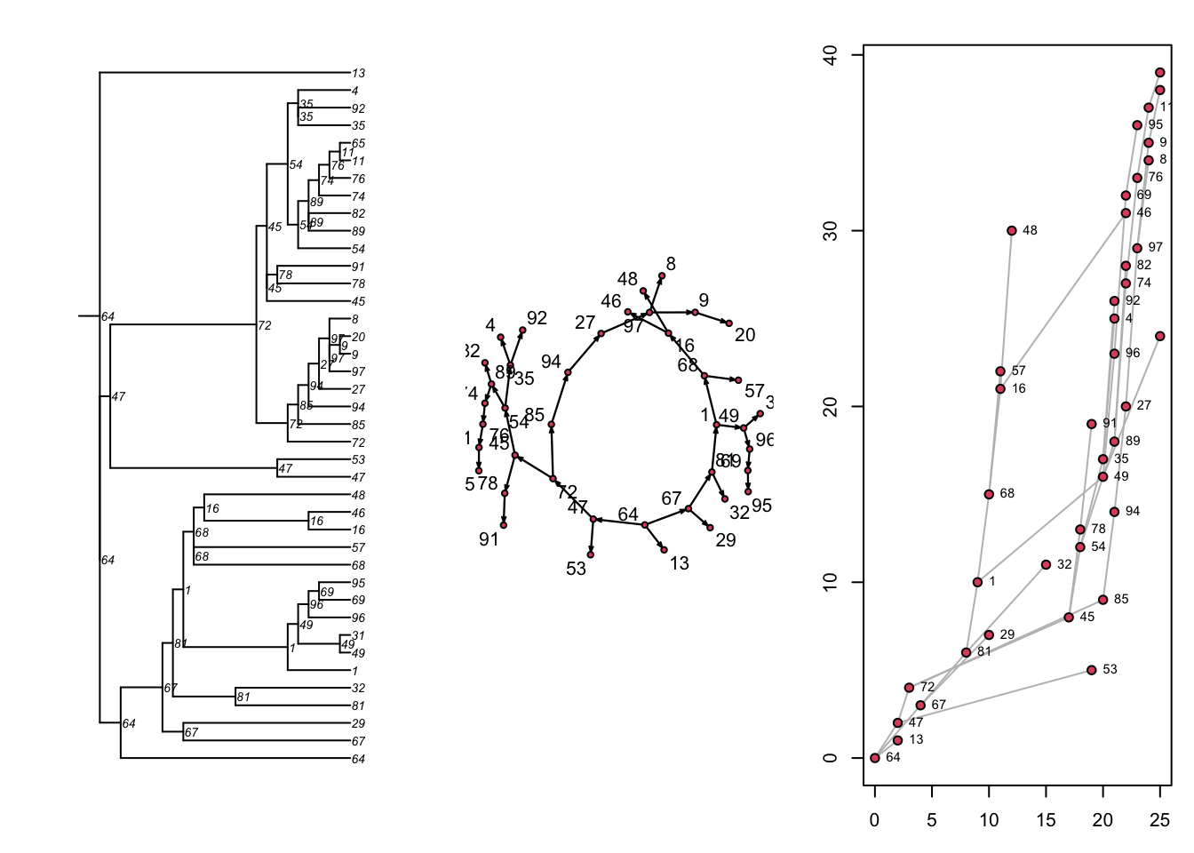
# ℹ 29 more rowsNext, there are three built-in visualizations for the transmission matrix, as shown here. Previously we converted the transmission matrix into a phylo class object and plotted a phylogram with the ape package. Here, we are showing that we can also plot this transmat object directly as a phylogram, and also as two related formats. Each show the time-directed chain of transmissions over time, starting with an initial seed. The middle plot is a directed network (showing who infected whom, here in a single large component because there was one seed). The right plot is a “transmission timeline” that plots the temporal time (the 25 time steps in our model) against generation time for transmissions.
Code

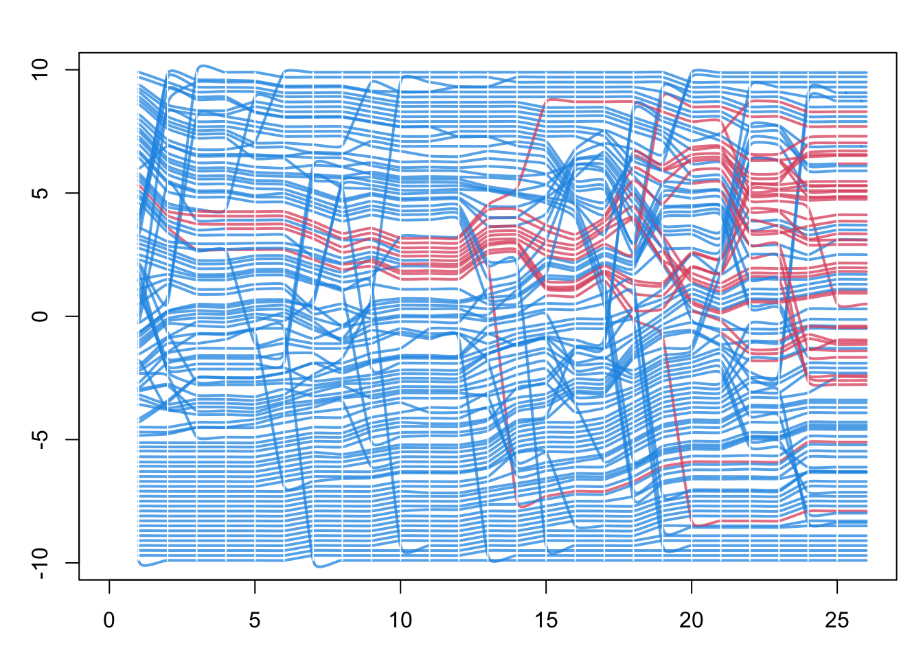
Finally, with the updated ndtv network object from above, we can plot a “proximity timeline” that shows the proximity of the nodes in directed temporal graph space, colored by disease status. Here the network is the full contact network, not just the transmission network of infected nodes. This helps identify the micro-outbreaks of infection that are occurring within sub-clusters of the network with greater closeness.
30.2.2.3 Dynamic Network Movie
There are lots of possibilities for how to model our networks over time. Here we animate the first 25 time steps of the simulation. To find out all the options, consult the main vignette for the ndtv package.
This step figures out where the nodes should be displayed in each animation frame. There are several dynamic layout options available, but we use the defaults here.
Finally, we render the animation and save it out to an HTML file using d3 Javascript. This makes for nice-looking animations within webpages. See the ndtv help for all the potential options in this step.
To embed movies into an RMarkdown document like this, we can set the output.mode accordingly.
30.3 Model 2: No Concurrency
Let’s return to the core network model and experiment with extra terms, and then run the movie again. Next we will add concurrent term in the model to control the number of nodes with overlapping partnerships. For reference, the expected number of concurrent nodes is a function of a Poisson distribution with the parameter equal to the mean degree (which is 2 x edges/N):
One helpful ERGM term is concurrent. This is the number of nodes with degree of 2 or higher. From the target stats above, next we can add a value for concurrent above or below the expected value of 19.1, and see how that plays out for our network movie. You may find that your model does not fit if the concurrent target stat is too high. That’s because you can’t have a huge number of concurrent persons if the mean degree (related to concurrency) is 0.8. In other words, the model terms and associated target statistics must be compatible.
30.3.1 Epidemic Model
In this example, we select an extreme concurrency statistic of 0 (no nodes exhibit concurrency).
Code
Warning: 'glpk' selected as the solver, but package 'Rglpk' is not available;
falling back to 'lpSolveAPI'. This should be fine unless the sample size and/or
the number of parameters is very big.We use the same epidemic parameters as above, but you can experiment with these too now.
30.3.2 Static Transmission Output
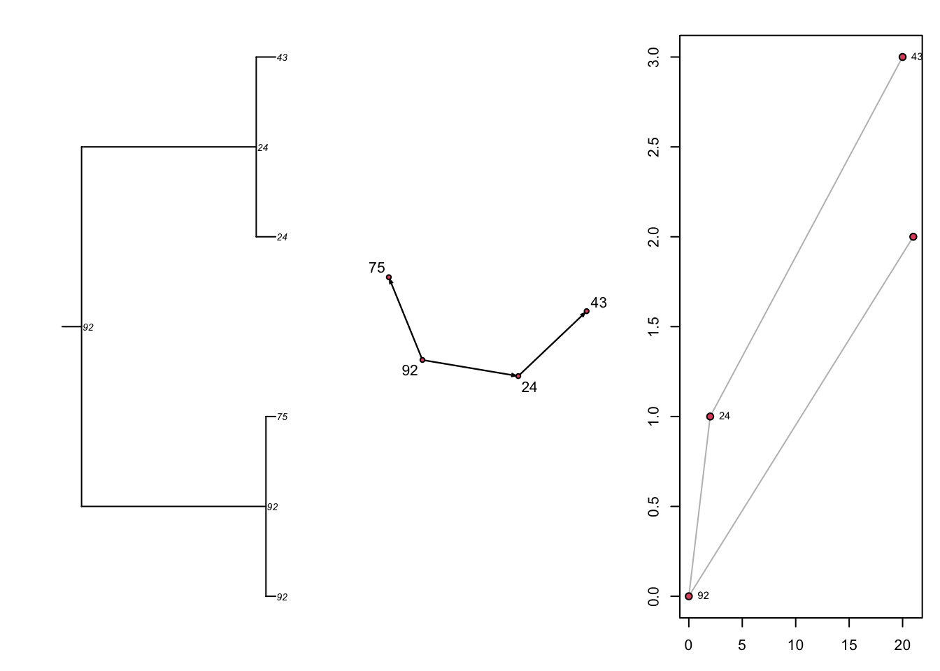
Let’s just look at what the static transmission outputs look like without network concurrency but with the same epidemic parameters. This network with much more sparse connectivity results in a transmission tree that is also sparser.
30.3.3 Dynamic Network Movie
We follow the same steps to make the movie. Notice here that nearly all nodes are connected within a dyad, and therefore that no concurrency implies few isolates given this relatively high mean degree (0.8). In fact, the logical maximum mean degree in a network with no concurrency would be 1.0. Notice how this “serial monogamy” constrains the speed of epidemic spread.
Code
nw <- get_network(sim)
nw <- color_tea(nw, verbose = FALSE)
compute.animation(nw, slice.par = slice.par)
render.d3movie(
  nw,
  render.par = render.par,
  plot.par = plot.par,
  vertex.cex = 0.9,
  vertex.col = "ndtvcol",
  edge.col = "darkgrey",
  vertex.border = "lightgrey",
  displaylabels = FALSE,
filename = paste0(getwd(), "/movie.html"))30.4 Model 3: Relational Duration
One feature of network models is to represent persistent relationships, in which there are repeated contacts between the same set of persons over time. This involves modeling the incident formation and persistence of edges over time. We can also model the extremes of relational duration to see its impact on epidemic potential.
30.4.1 Model 3a: Very Long Durations
Here we use the same model as Model 1, but set the duration to 100,000 time steps. This effectively makes all edges fixed over the 25 simulation time steps.
We use the same epidemic parameters as above.
We follow the same steps to make the movie. Nothing much happening, even with a transmission probability of 100%.
Code
nw <- get_network(sim)
nw <- color_tea(nw, verbose = FALSE)
compute.animation(nw, slice.par = slice.par)
render.d3movie(
  nw,
  render.par = render.par,
  plot.par = plot.par,
  vertex.cex = 0.9,
  vertex.col = "ndtvcol",
  edge.col = "darkgrey",
  vertex.border = "lightgrey",
  displaylabels = FALSE,
filename = paste0(getwd(), "/movie.html"))30.4.2 Model 3b: Short-Duration Contacts
Here we use the same model as Model 1, but set the duration to 2 time steps. This makes edges randomly disolve with high probabilities at each time step.
We use the same epidemic parameters as above.
Yikes! There is not only massive turnover in the edges at each time step (which makes the visualization a jumble of moving nodes), but the epidemic quickly reaches a saturation point.
Code
nw <- get_network(sim)
nw <- color_tea(nw, verbose = FALSE)
compute.animation(nw, slice.par = slice.par)
render.d3movie(
  nw,
  render.par = render.par,
  plot.par = plot.par,
  vertex.cex = 0.9,
  vertex.col = "ndtvcol",
  edge.col = "darkgrey",
  vertex.border = "lightgrey",
  displaylabels = FALSE,
filename = paste0(getwd(), "/movie.html"))30.5 Model 4: Triangles
Next let’s try another model where we add extra “triangles”: clusters of three people connected together in a local group. The gwesp term allows us to do this without problems of model degeneracy (see Day 2 materials). The null value for the target statistic is less than 1, so let’s ramp it up a bit and see what happens. We will recycle the same epidemic parameters from the model above.
We follow the same steps to make the movie. Notice the distinct triangle formation in the network edges. Are triangles associated with faster or slower epidemic spread?
Code
nw <- get_network(sim)
nw <- color_tea(nw, verbose = FALSE)
compute.animation(nw, slice.par = slice.par)
render.d3movie(
  nw,
  render.par = render.par,
  plot.par = plot.par,
  vertex.cex = 0.9,
  vertex.col = "ndtvcol",
  edge.col = "darkgrey",
  vertex.border = "lightgrey",
  displaylabels = FALSE,
filename = paste0(getwd(), "/movie.html"))30.6 Model 5: Extra Nodal Attributes
Finally, we show an example of how to work with additional vertex attributes within the model. Unlike in today’s Session 5 tutorial, which used the special group attribute, here we show how to use other (non-special) attributes in combination.
In this model, we want to parameterize a network model in which age and race/ethnicity attributes are represented. Race will be a single binary variable (0 and 1), whereas age will be an integer in years between 18 and 50. We use R’s built-in random sampling functions to generate values for these attributes and then set them on the network object.
Code
 Network attributes:
  vertices = 100
  directed = FALSE
  hyper = FALSE
  loops = FALSE
  multiple = FALSE
  bipartite = FALSE
  total edges= 0
    missing edges= 0
    non-missing edges= 0

 Vertex attribute names:
    age race vertex.names

No edge attributes
This will be the most complex TERGM formula that we have seen so far. It introduces a couple of new ERGM terms for Day 3 and chains them all together in a single model. We start with an edges term with an associated target statistic of 50 (so an overall mean degree of 1). Next is a nodematch("race") term that specifies that 40 of those 50 edges are within the same race group. After that the nodefactor("race") term allows the mean degree to vary by race. We will work on parameterizing this statistic further in Day 4, but with a target statistic of 70, this means that the race=1 group has a mean degree of 70/50=1.4 (the nodefactor term has a default reference group that is the lowest value of the referenced attribute). Next, the absdiff term is a mixing term, like nodematch, but for a continuous attribute (like age). The target statistic of 100 represents the sum of the absolute differences in the age attribute across all dyads in the network; with 50 edges, this means that dyads are on average 2 years apart in age (in either direction). Finally, we include a concurrent term to parameterize network degree. In the dissolution model, we specify that the average duration of edges is 20 time steps in relations not matched on race, and 10 time steps in relations matched on race.
Phew! The epidemic model is simple, and parameterized as before.
The first steps of making the network movie are the same as before.
But to visualize race and age in the movie, we will extract the attributes back from the network object. And then scale them for appropriate visuals. We convert race into two numbers, 4 and 50, the will represent the number of sides in the node (so: a square and a circle). We scale age by a factor of 1/25 to allow the node size to be a simple function of age.
And here’s our final movie!


