23 Lab
In this lab, you can work to simulate your first network-based epidemic model! The goal here will be to take the concepts and technical methods you have learned so far to extend the model in the SIS tutorial. The specific learning objectives for this lab are to:
23.1 Setup
Once you are ready, start out by clearing your R object environment, to make sure that you do not have any objects lingering from the tutorial. This can be accomplished with:
When you are plotting your figures below, you can switch between single and double panel plots with the graphical parameter mfrow, like this:
To modify the plot margins, you can use the mar parameter (this may need to be set after plotting the networks with zero margins):
The four numbers correspond to the amount of space on the right, bottom, left, and top, in that order.
23.2 Lab Steps
The tutorial in Module 4 used a parameter for concurrency (degree of 2+) based on an estimate that 22% of the population had overlapping relations. What would happen to the epidemic trajectory relative to the outcomes presented in the tutorial if concurrency was prohibited but the mean degree remained constant?
- Implement this in the network model target statistics, then estimate the TERGM (
netest), and diagnose it (netdx). Do you need thedegrangeterm in the model now? How does the degree distribution (count of nodes with degree 0, 1, 2, 3, 4…) change here compared to the tutorial? - Run the SIS epidemic model using the same parameters as in the tutorial. 5 simulations over 500 time steps is fine. Feel free to use the multi-core capabilities of your computer during
netsimby specifying anncoresvalue (the default is 1). - Summarize the outcomes visually (plot the prevalence and incidence) and numerically (you can use the summary function). What happens to the epidemic trajectory compared to the tutorial?
- Plot a network diagram from a simulation at the beginning and end of the time series.
23.3 Lab Questions
After you have completed running the models above, please consider the following conceptual questions:
- What are the implications of the changes to the degree distribution when the mean degree is held constant, as it is here in the lab? Do you think this is realistic for human social relations, and if not, how would you change the model parameters above in a follow-up model?
- What are the reasons for the changes in the epidemic trajectory when concurrency was prohibited? How might this differ for another epidemic that might have different biological properties (e.g., different transmission probability or recovery rate)? How would you test this in a follow-up model?
23.4 Additional Exploration
After that, you could explore the model by changing:
- the average duration of partnerships, up or down
- one or all of the epidemic parameters in the model
- change it to an SI model (
type = "SI", remove therec.rateparameter inparam.net) - change it to an SIR model (
type = "SIR", addr.num = 0ininit.net) - add a simple vaccine intervention
