Tuberculosis in Households and the Community

A full TB model on a three-layer contact network: households as cliques built with netclique() and kept intact through births, deaths, and people leaving home, plus regular and casual community contacts as TERGMs. Fast and slow latency, reinfection under partial protection, age-specific natural history, and heavy-tailed infectiousness. It asks why households carry a small share of transmission despite a large share of contact time, how the persistence of ties changes transmission, and what household contact investigation with preventive therapy achieves next to community-wide and random screening.

Overview

Tuberculosis (TB) is transmitted through shared air, most often over long periods of contact, and most people infected with Mycobacterium tuberculosis never develop disease. Those who do usually progress within the first year or two after infection, a smaller number decades later, and a person with active TB can transmit for many months before diagnosis. In high-burden settings, recent transmission, including reinfection of people already infected, accounts for most incident disease.

Household members share more contact time than any other set of people, and household contact investigation, in which the co-residents of every newly diagnosed person are screened for TB and offered preventive treatment, is a core WHO recommendation. Yet molecular and genomic studies in high-burden settings attribute only 8 to 19% of transmission to household contacts (Verver et al. 2004; Glynn et al. 2015; Middelkoop et al. 2015), and in a Western Cape contact survey households held 36% of adults’ contact time but, in a model built on those data, only 13% of disease (McCreesh and White 2018). How much transmission happens at home, and why it is less than contact time suggests, decides how much a household-targeted program can accomplish.

This example builds a TB model to examine that question. It has three features that no other Gallery example combines:

1. A household clique layer in an open population. Households are cliques built with netclique(). Newborns join a household through the layer’s arrival rule, the dead leave with their edges, and young adults leave home to form new households through move_to_group(). Two TERGM layers carry non-household contacts: regular contacts (coworkers, classmates, friends) that last about a year, and casual contacts (transport, markets, shops) that are redrawn every month. Each contact layer is weighted by its contact time, taken from a Western Cape contact survey.

2. A TB natural history with age structure. The disease states follow the compartmental model of Rothman et al. (2026): early (fast) and late (slow) latent infection, reinfection under the partial protection of prior infection, active disease, treatment, and relapse. To these the example adds self-cure, clearance of late latent infection, age-specific progression and infectiousness for children and adults, births and deaths over decades, and heavy-tailed variation in how infectious each case is.

3. Two experiments that need a network. Part 1 holds contact time and per-contact-hour risk fixed and rearranges the same contacts: households as they are, regular contacts redrawn every month, and household contact time spread across random partners redrawn every month. This separates what the persistence and clustering of ties do to transmission from what the amount of contact does. Part 2 resumes the baseline and compares household contact investigation, with and without preventive therapy, against community-wide screening of adults and against an equal-effort comparator that screens the same number of people chosen at random, which isolates the value of the household link.

The policy question is the one asked of TB programs in high-burden settings: what does household contact investigation achieve, per person screened and for the population, when most transmission happens outside the home?

NoteEpiModel features used here

• netclique() for a household layer of cliques, with arrivals = "join" and a custom arrivals.FUN that places newborns; assign_groups() to build households around existing ages; and move_to_group() to move people between households during a simulation.
• TERGM layers with a fully targeted nodemix mixing matrix, and per-layer control.simulate.formula.tergm() settings passed with multilayer().
• Custom modules with an explicit module.order, transmission on each layer weighted by contact-hours, and set_transmat() records with extra columns.
• A burn-in saved with save.run = TRUE, and intervention scenarios resumed from it one simulation at a time with get_sims(), use_scenario(), and merge().
• Monte Carlo intervals on every model output.

NoteHow this relates to other TB models

The TB models most used for policy, including TIME Impact, Tabby2, AuTuMN, Optima TB, and the models in the TB Modelling and Analysis Consortium comparisons, are population-level compartmental models, as is the Rothman et al. (2026) model from which this example takes its disease structure. They represent contact through mixing matrices and are built to project incidence, mortality, and costs for a country. Household structure appears in theoretical models of close and casual contact (Aparicio et al. 2000) and in research individual-based and network models (Cohen et al. 2007; Kasaie et al. 2014; McCreesh and White 2018; Havumaki et al. 2021), nearly all of which hold community ties fixed; one built in EpiModel used static village networks (Pando et al. 2023). This example trades calibration to a country for an explicit multilayer network in which households are real groups, community ties turn over at a rate the modeler chooses, and every transmission is attributed to a layer. Its setting is a generic high-burden one without HIV, its parameters are illustrative, and it is not calibrated to surveillance data. Treat it as a template for building a TB network model, not as a projection for any place.

TipDownload and run the standalone scripts

• model.R: main simulation script
• module-fx.R: custom module functions

model.R sources module-fx.R from examples/tuberculosis/ when run from the repository root and from the working directory otherwise. Sourcing the script interactively uses the full settings on this page (N = 20000, ten simulations, a 50-year burn-in for each of three contact structures, five 10-year intervention scenarios), which take about half an hour on five cores. Rscript is not interactive and uses small continuous-integration settings whose results are not meant to be interpreted; to get the full settings from the command line, pass R code that defines run_full as the first argument:

Rscript model.R "run_full <- TRUE"

Model Structure

Disease states

Status	Description	Can be infected?	Infectious?
s	Never infected	yes, full susceptibility	no
e	Early latent infection, the months after infection when the risk of disease is highest	no	no
l	Late latent infection, with a small lifelong risk of reactivation	yes, at 21% of full susceptibility	no
c	Infection cleared, spontaneously or by preventive therapy; no risk of reactivation	yes, at 21% of full susceptibility	no
i	Active TB, not yet diagnosed	no	yes, by age and case
t	On treatment (six months)	no	no
r	Recovered from TB (treated or self-cured), with a risk of relapse in the first years	yes, full susceptibility	no

flowchart LR
    S["<b>s</b><br/>never infected"] -->|infection| E["<b>e</b><br/>early latent"]
    E -->|early progression| I["<b>i</b><br/>active TB"]
    E -->|stabilization| L["<b>l</b><br/>late latent"]
    L -->|reactivation| I
    L -->|clearance| C["<b>c</b><br/>cleared"]
    L -->|reinfection| E
    C -->|reinfection| E
    I -->|diagnosis| T["<b>t</b><br/>treatment"]
    I -->|self-cure| R["<b>r</b><br/>recovered"]
    T -->|cure| R
    T -->|failure or loss| I
    R -->|relapse| I
    R -->|stabilization| L
    R -->|reinfection| E

    style S fill:#3498db,color:#fff
    style E fill:#9b59b6,color:#fff
    style L fill:#8e44ad,color:#fff
    style C fill:#7f8c8d,color:#fff
    style I fill:#e74c3c,color:#fff
    style T fill:#f39c12,color:#fff
    style R fill:#27ae60,color:#fff

TB deaths occur from active TB and during treatment; background mortality applies to everyone. Screening programs (Part 2) move people with active TB to treatment and people with latent infection to the cleared state.

Two features of this structure carry most of the TB-specific behavior. First, infection is not immunity: a person with latent or cleared infection can be reinfected, but has a 79% lower risk of the disease that reinfection would otherwise cause (Andrews et al. 2012). The model applies this as a 79% lower probability that an exposure establishes a new infection, after which the person passes through early latency again. Rothman et al. applied this protection only to people who had recovered from TB; here it applies to everyone with prior infection, as in the cohorts it was measured in, and people who have recovered from TB have none, since disease from reinfection after cure occurs at four times the rate of new TB (Verver et al. 2005). Second, untreated disease ends in one of three ways: diagnosis and treatment, self-cure, or death. In the Rothman et al. model of the United States, treatment and death are the only exits from disease; in a high-burden setting the months to years of undiagnosed disease are where transmission happens.

Age

Age is continuous and advances each month. Natural history uses three bands, 0 to 4, 5 to 14, and 15 and older, because the risk of disease after infection is U-shaped in childhood: high in young children, low in school-age children, and adult-like from adolescence (Marais et al. 2004; Martinez et al. 2020). Children under 10 are treated as non-infectious and those 10 to 14 as half as infectious as adults, a modeling convention reflecting that childhood TB is usually paucibacillary. The contact layers use a two-group attribute, agegrp ("child" under 15, "adult" 15 and older), for their mixing terms.

Contact layers

Layer	Construction	Tie duration	Contact time per adult per day
household	netclique() on the household id: every pair of co-residents	as long as they live together	17.0 hours
regular	TERGM with a full age-mixing matrix	mean 12 months	6.0 hours
casual	TERGM with a full age-mixing matrix	1 month (redrawn every step)	24.2 hours

The daily contact times are the person-hours per day that adults in the Western Cape spent with household members, repeated non-household contacts, and non-repeated contacts (McCreesh and White 2018). Each edge on a layer carries that layer’s contact time divided by the adult mean degree on the layer, so an adult with the average number of contacts has the reported daily contact time on each layer. The probability that an edge transmits in a month is \(1 - \exp(-\beta h_k m_i a_i s_j)\) for per-contact-hour risk \(\beta\), monthly hours per edge \(h_k\) on layer \(k\), the case’s individual infectiousness \(m_i\) and age multiplier \(a_i\), and the susceptibility \(s_j\) of the other person. In the transmission probability the layers differ only in their contact time per edge; beyond that, they differ in how their ties are arranged and how long those ties last.

Setup

suppressMessages(library(EpiModel))

# These are the full settings of the standalone model.R. Time steps are
# months: a 50-year burn-in, then 10 years of intervention scenarios.
N <- 20000
nsims <- 10
ncores <- 5
burnin <- 600
horizon <- 120

# The custom modules used in control.net() and the netclique arrival rule.
# The excerpts shown under "Custom Modules" are pulled from this file.
source("module-fx.R")

Population and Households

A stationary population

The model runs for decades, so the population has births and deaths and its age structure has to hold still while it does. Background mortality is a step function of age, chosen so that the stationary population has a life expectancy at birth of about 60 years and about a quarter of its members under 15, close to South Africa (26% under 15). Ages are drawn from that stationary distribution, and births at a per-capita rate of \(1/e_0\) keep the population’s size and age structure steady in expectation, apart from TB deaths, which shrink it by a few percent over the decades of a run.

mort.breaks <- c(0, 1, 5, 15, 30, 45, 60, 70, 80)
mort.rates <- c(0.025, 0.002, 0.0012, 0.004, 0.009, 0.020, 0.040, 0.080, 0.180)
age_grid <- seq(0, 100 - 1 / 12, by = 1 / 12)
mort_grid <- mort.rates[findInterval(age_grid, mort.breaks)]
surv <- exp(-cumsum(c(0, head(mort_grid, -1) / 12)))
e0 <- sum(surv) / 12

set.seed(12)
age <- sample(age_grid, N, replace = TRUE, prob = surv) + runif(N, 0, 1 / 12)
agegrp <- ifelse(age < 15, "child", "adult")
c(life_expectancy = round(e0, 1), pct_under_15 = round(100 * mean(age < 15), 1))

life_expectancy    pct_under_15 
           59.7            24.3 

Households with assign_groups()

assign_groups(), which comes with netclique(), builds household ids for a population whose attributes already exist: it draws household sizes from a target distribution, places one adult in each household, puts children in the open slots of households that have an adult, and fills the rest. The size distribution below has a mean of about 3.3 people and 22% single-person households, close to South Africa’s census (3.5 and 26%).

hh_size_dist <- c("1" = 0.22, "2" = 0.18, "3" = 0.17, "4" = 0.16, "5" = 0.11,
                  "6" = 0.08, "7" = 0.05, "8" = 0.03)
hh_id <- assign_groups(hh_size_dist, role = agegrp, anchor = "adult",
                       dependent = "child")
table(household_size = tabulate(hh_id))

household_size
   1    2    3    4    5    6    7    8 
1316 1056 1027  977  637  476  314  168 

The household layer with netclique()

netclique() turns a grouping attribute into a network layer in which every pair of nodes sharing a value is an edge. It returns an object that goes into the layer list passed to netsim() alongside netest() fits; the network resimulation skips it, and the infection module reads it with get_edgelist() like any other layer. Every vertex attribute the modules need is set on the one base network from which all layers are built, because netsim() reads nodal attributes from the first layer.

nw <- network_initialize(N)
nw <- set_vertex_attribute(nw, "age", age)
nw <- set_vertex_attribute(nw, "agegrp", agegrp)
nw <- set_vertex_attribute(nw, "hh_id", hh_id)

1est_hh <- netclique(nw, group.attr = "hh_id", arrivals = "join",
                    arrivals.FUN = newborn_household)
print(est_hh, by = "agegrp")

1

arrivals = "join" connects each arriving node to every member of an existing household. By default the household is drawn in proportion to its size; arrivals.FUN replaces that draw with a rule of our own.

EpiModel Clique Network Layer
=======================
Model class: netclique
Grouping attribute: hh_id

Layer Summary
-----------------------
Nodes: 20000
Groups: 5971
Edges: 34807
Mean degree: 3.481
Isolates: 1316

Group Size Distribution
-----------------------
                                         
size      1    2    3   4   5   6   7   8
groups 1316 1056 1027 977 637 476 314 168

Mean Degree by `agegrp`
-----------------------
adult child 
3.321 3.976 

Arrivals: join (group chosen by arrivals.FUN)

The arrival rule places each newborn in the household of a randomly chosen adult aged 15 to 49, so every child is born into a household with an adult of childbearing age:

newborn_household <- function(dat, at, new_ids, network) {
  active <- get_attr(dat, "active")
  age <- get_attr(dat, "age")
  hh_id <- get_attr(dat, "hh_id")
  parents <- setdiff(which(active == 1 & !is.na(hh_id) & age >= 15 & age < 50),
                     new_ids)
  if (length(parents) == 0) {
    return(rep(NA, length(new_ids)))
  }
  hh_id[parents[sample.int(length(parents), length(new_ids), replace = TRUE)]]
}

NoteWhy a clique layer, and why not a stored edgelist

A household edgelist built once and passed to netsim() as a parameter works for a closed population over one season. With births and deaths that approach breaks. Under tergmLite, EpiModel deletes the departed from every attribute vector and edgelist at the end of each step and shifts the positions of everyone after them, so a stored edgelist points at the wrong people after the first death: in a test of this model’s demography, half of the stored household pairs joined people in different households after 100 months. A netclique() layer is updated in step with the attributes. The departed leave with their edges, a household whose last member dies ceases to exist, arrivals are placed by the layer’s rule, and the layer survives a restart from a saved burn-in, which Part 2 relies on.

Leaving home: move_to_group()

Births only add people to existing households, and deaths only remove them. Left alone, households grow and their number shrinks: in a test with a similar demography and no moves, the size of the household the average person lives in rose from 4.4 to 7.1 over 50 years. People already in the population also have to change households. The households module (below) lets young adults leave home to form new households and moves children left without an adult into another household, both through move_to_group(), which sets the household id and rewires the clique layer in one step. Setting hh_id with set_attr() alone would change the attribute but leave the old household edges in place.

Community Layers

The regular and casual layers are TERGMs whose formation model is ~edges + nodemix("agegrp"), with every cell of the child-adult mixing matrix targeted, as in the RSV example. Each profile entry a.b is the mean number of b-partners per a-node: adults have about five regular contacts at a time and six new casual contacts each month; children have six regular contacts, mostly other children at school, and three casual contacts a month, half of them adults.

counts <- table(agegrp)
cells <- sub("^mix\\.agegrp\\.", "",
             names(summary(nw ~ nodemix("agegrp", levels2 = TRUE))))
mix_targets <- function(profile) {
  out <- setNames(numeric(length(cells)), cells)
  for (nm in names(profile)) {
    ab <- strsplit(nm, ".", fixed = TRUE)[[1]]
    n_a <- as.numeric(counts[ab[1]])
    e <- if (ab[1] == ab[2]) n_a * profile[[nm]] / 2 else n_a * profile[[nm]]
    cell <- paste(sort(ab), collapse = ".")
    out[cell] <- out[cell] + e
  }
  pmax(round(out), 1)
}
reg_profile <- c(adult.adult = 4.6, child.adult = 1.0, child.child = 5.0)
cas_profile <- c(adult.adult = 5.5, child.adult = 1.5, child.child = 1.5)
reg_targets <- mix_targets(reg_profile)
cas_targets <- mix_targets(cas_profile)

formation <- ~edges + nodemix("agegrp", levels2 = -1)
san_ctrl <- control.ergm(SAN = control.san(SAN.maxit = 20, SAN.nsteps = 2^21))
d.rate <- 1 / e0 / 12

est_reg <- netest(nw, formation,
                  target.stats = c(sum(reg_targets), as.numeric(reg_targets[-1])),
1                  coef.diss = dissolution_coefs(~offset(edges), duration = 12,
                                                d.rate = d.rate),
                  set.control.ergm = san_ctrl, verbose = FALSE)
est_cas <- netest(nw, formation,
                  target.stats = c(sum(cas_targets), as.numeric(cas_targets[-1])),
2                  coef.diss = dissolution_coefs(~offset(edges), duration = 1),
                  set.control.ergm = san_ctrl, verbose = FALSE)

1

Regular ties last 12 months on average. d.rate adjusts the dissolution coefficient for ties that end because a partner dies.

2

Casual ties last one month: every step brings a new set.

Simulating the community layers faithfully

tergm simulates each time step with a Markov chain whose default length is far too short for these two layers. With the default chain, about half of the casual ties survived from one month to the next, although the model says every casual tie lasts one month, and the regular layer’s children-with-children cell settled about 20% below its target, because proposals rarely land on the small set of child-child dyads. Both problems largely go away with a chain long enough to visit every tie, which scales with the number of edges and hence with N: carried-over casual ties fall to about 3% a month. The longer chains about double the time spent simulating the two layers.

mcmc <- function(steps) {
  control.simulate.formula.tergm(MCMC.burnin.min = steps, MCMC.burnin.max = steps)
}
tergm_persist <- mcmc(20 * N)
tergm_redraw <- mcmc(25 * N)

Diagnostics and contact time

The regular layer is simulated dynamically, which checks both its degree by age group and its mean tie duration; the casual layer’s ties last one step, so its formation model is checked with static simulations. The household layer’s degree is read directly from the cliques.

dx_reg <- netdx(est_reg, nsims = 2, nsteps = 60, set.control.tergm = tergm_persist,
                nwstats.formula = ~edges + nodefactor("agegrp", levels = TRUE),
                verbose = FALSE)
dx_cas <- netdx(est_cas, nsims = 10, dynamic = FALSE,
                nwstats.formula = ~edges + nodefactor("agegrp", levels = TRUE),
                verbose = FALSE)
dx_reg$stats.table.duration

      Target Sim Mean   Pct Diff     Sim SE    Z Score SD(Sim Means)
edges     12  11.9835 -0.1374642 0.01969739 -0.8374562    0.01211522
      SD(Statistic)
edges    0.04802619

realized_degree <- function(dx) {
  st <- colMeans(do.call(rbind, lapply(dx$stats, as.matrix)))
  st[paste0("nodefactor.agegrp.", c("adult", "child"))] /
    as.numeric(counts[c("adult", "child")])
}

hh_el <- as.edgelist(est_hh$newnetwork)
hh_deg <- tabulate(c(hh_el), nbins = N)
deg_tbl <- rbind(
  household = tapply(hh_deg, agegrp, mean),
  regular = c(adult = 2 * reg_targets[["adult.adult"]] + reg_targets[["adult.child"]],
              child = reg_targets[["adult.child"]] + 2 * reg_targets[["child.child"]]) /
    as.numeric(counts[c("adult", "child")]),
  casual = c(adult = 2 * cas_targets[["adult.adult"]] + cas_targets[["adult.child"]],
             child = cas_targets[["adult.child"]] + 2 * cas_targets[["child.child"]]) /
    as.numeric(counts[c("adult", "child")])
)
deg_show <- cbind(deg_tbl, rbind(household = deg_tbl["household", ],
                                 regular = realized_degree(dx_reg),
                                 casual = realized_degree(dx_cas)))
colnames(deg_show) <- c("adult, target", "child, target",
                        "adult, simulated", "child, simulated")
knitr::kable(round(deg_show, 2),
             caption = "Mean degree by age group and layer: targets and values from simulations of the fitted models (the household layer is fixed by the cliques)")

Mean degree by age group and layer: targets and values from simulations of the fitted models (the household layer is fixed by the cliques)

	adult, target	child, target	adult, simulated	child, simulated
household	3.32	3.98	3.32	3.98
regular	4.92	6.00	4.90	5.95
casual	5.98	3.00	5.94	2.99

Contact time converts degree into exposure. McCreesh and White (2018) report that adults in the Western Cape spent about 17.0 person-hours a day with household members, 6.0 with repeated non-household contacts, and 24.2 with non-repeated contacts. Dividing each by the adult mean degree on its layer gives the monthly hours carried by one edge:

hours_day <- c(household = 17.0, regular = 6.0, casual = 24.2)
layer_hours <- hours_day / deg_tbl[, "adult"] * 365.25 / 12
round(layer_hours, 1)

household   regular    casual 
    155.8      37.1     123.1 

A household edge carries 156 hours a month, about 5.1 hours a day with each co-resident; a regular edge 37 hours; a casual edge 123. A casual edge is an abstraction: the roughly 240 people an adult meets briefly in a month, in the Western Cape survey, are pooled into about six edges that are replaced every month. That reproduces the total casual contact time and the fact that it is spent with ever-changing people, but an edge can transmit only once in a month, so the pooling caps how many people a highly infectious case can infect through casual contact. The Simplifications callout below says what that does to the results.

Custom Modules

Nine custom modules run in each monthly step: init_tb (one-shot setup of the TB states), aging, infect, progress (natural history and passive diagnosis), screen (the Part 2 programs), deaths, births, households (leaving home), and tally (summary counts). Full code is in module-fx.R; the parts that carry the model’s logic are below.

infect: transmission weighted by contact time, on every layer

The module walks each layer’s current edgelist, whether the layer is a clique or a TERGM, and gives each discordant edge its own probability of transmission. Nothing downstream of get_edgelist() depends on the kind of layer.

1infness[ids_i] <- inf_mult[ids_i] *
  age.mult[findInterval(age[ids_i], age.breaks)]
2sus[status == "s"] <- 1
sus[status %in% c("l", "c")] <- sus.latent
sus[status == "r"] <- sus.recovered

for (k in seq_along(hours)) {
  if (hours[k] == 0) next
3  el <- get_edgelist(dat, network = k)
  a <- el[, 1]
  b <- el[, 2]
  fwd <- infness[a] > 0 & sus[b] > 0
  rev <- infness[b] > 0 & sus[a] > 0
  inf <- c(a[fwd], b[rev])
  rec <- c(b[fwd], a[rev])
4  p <- 1 - exp(-beta * hours[k] * infness[inf] * sus[rec])
  hit <- which(runif(length(p)) < p)
  if (length(hit) > 0) {
    del <- rbind(del, data.frame(sus = rec[hit], inf = inf[hit], layer = k))
  }
}
5del <- del[sample.int(nrow(del)), , drop = FALSE]
del <- del[!duplicated(del$sus), , drop = FALSE]

1

Infectiousness. Each case’s multiplier inf_mult is drawn when the episode begins, from a gamma distribution with mean 1 and shape inf.k = 0.15; the age multiplier is 0 under 10, 0.5 at 10 to 14, and 1 from 15.

2

Susceptibility. Full for the never infected and for people who have recovered from TB; 0.21 for people with latent or cleared infection.

3

One call for any layer. Layer 1 is the netclique layer, layers 2 and 3 the TERGMs; in the Part 1 variant with redrawn households a fourth layer is added and the clique layer’s hours are set to zero.

4

Contact-hour dose. The probability rises with contact time and saturates: an edge cannot transmit more than once, however long or intense the contact.

5

Competing exposures. A node infected on several edges in the same step is infected once, and its infector, and so its layer, is drawn at random among the successes. The transmission record keeps the layer, both ages, the recipient’s prior state, and the infector’s unique id, from which the concentration of transmission among cases is computed.

progress: competing risks at a monthly step

Most TB states have more than one exit. The module draws whether a node leaves a state in the month from the sum of the exit rates, and then which exit in proportion to the rates, so the share of people taking each route is exact at a monthly step rather than depending on the order in which transitions are checked.

exits <- function(ids, rates) {
  rates <- matrix(rates, nrow = length(ids))
  tot <- rowSums(rates)
  out <- integer(length(ids))
1  go <- which(u1[ids] < 1 - exp(-tot / 12))
  if (length(go) > 0) {
    out[go] <- 1L
    cum <- 0
2    for (j in seq_len(ncol(rates) - 1)) {
      cum <- cum + rates[go, j] / tot[go]
      out[go] <- out[go] + (u2[ids[go]] > cum)
    }
  }
  out
}

## early latent: progression or stabilization, by age band
ids <- which(active == 1 & status0 == "e" & infTime < at)
x <- exits(ids, cbind(prog.early[band[ids]], stab.early[band[ids]]))

## active TB: diagnosis, TB death, or self-cure
ids <- which(active == 1 & status0 == "i")
x <- exits(ids, cbind(diag.rate, tb.mort[band[ids]], self.cure))

1

Annual rates are converted to a monthly probability of leaving the state.

2

The exit taken is drawn in proportion to the rates.

screen: one package for household and random screening

Household contact investigation and the equal-effort random arm deliver the same package, so it is written once. Screened people with active TB are found with an age-specific sensitivity and start treatment; eligible people who are not found to have TB are offered preventive therapy (TPT), and a completed course clears early or late latent infection.

package <- function(ids, status, txTime, dxTime) {
  sens <- ifelse(age[ids] < 15, screen.sens[1], screen.sens[2])
  found <- ids[status[ids] == "i" & runif(length(ids)) < sens]
  status[found] <- "t"
  txTime[found] <- at
  dxTime[found] <- at
  elig <- setdiff(ids[age[ids] < tpt.age.max & status[ids] != "t"], found)
  started <- elig[runif(length(elig)) < tpt.start]
  completed <- started[runif(length(started)) < tpt.complete]
1  latent <- completed[status[completed] %in% c("e", "l")]
  cleared <- latent[runif(length(latent)) < tpt.eff]
  status[cleared] <- "c"
  ...
}

2index <- which(is_active & !is.na(dxTime) & dxTime == at)
idx_hh <- unique(hh_id[index])
contacts <- setdiff(which(is_active & hh_id %in% idx_hh & !is.na(hh_id)), index)
3reached_hh <- idx_hh[runif(length(idx_hh)) < hhci.reach]
ev <- contacts[hh_id[contacts] %in% reached_hh & status[contacts] != "t"]
ev <- ev[runif(length(ev)) < hhci.eval]
out <- package(ev, status, txTime, dxTime)

1

TPT acts only on people who are infected, but it is offered without testing for infection, as WHO recommends for household contacts under 5 and allows for older contacts. A cleared infection keeps the partial protection of prior infection; TPT adds none of its own, so a treated contact can be reinfected.

2

Index cases are everyone diagnosed in this step, whether passively or by a screening program.

3

The household id makes “the co-residents of a newly diagnosed person” a set the module can find directly.

The module also records, for every index case, the state of each co-resident at the moment of diagnosis. That is the model’s counterpart of the household contact studies used to check it below, and it is recorded in every scenario whether or not a program is running.

households: leaving home with move_to_group()

elig <- which(active == 1 & !is.na(hh_id) & age >= leave.ages[1] &
                age < leave.ages[2] & size >= 3 & adults >= 2)
leavers <- elig[runif(length(elig)) < leave.rate]
if (length(leavers) > 0) {
  leavers <- leavers[sample.int(length(leavers))]
1  new_ids <- max(hh_id, na.rm = TRUE) + ceiling(seq_along(leavers) / 2)
2  dat <- move_to_group(dat, ids = leavers, group = new_ids)
  hh_id <- get_attr(dat, "hh_id")
}

1

Leavers are paired at random into new two-person households, and an odd leaver lives alone. Unused ids start new households.

2

move_to_group() removes each mover’s household edges and connects the mover to every member of the new household, including the partner who moved with them.

The same function moves children whose household has no one aged 15 or older left, together, into the household of a randomly chosen adult.

births: append every attribute

dat <- append_core_attr(dat, at, n_new)
dat <- append_attr(dat, "status", "s", n_new)
dat <- append_attr(dat, "age", 0, n_new)
dat <- append_attr(dat, "agegrp", "child", n_new)
1dat <- append_attr(dat, "hh_id", NA, n_new)
dat <- append_attr(dat, "infTime", NA_integer_, n_new)
dat <- append_attr(dat, "infType", NA_character_, n_new)
dat <- append_attr(dat, "inf_mult", NA_real_, n_new)
dat <- append_attr(dat, "txTime", NA_integer_, n_new)
dat <- append_attr(dat, "dxTime", NA_integer_, n_new)
dat <- append_attr(dat, "hhcTime", NA_integer_, n_new)

1

The household is left missing here and set by the clique layer’s arrival rule, newborn_household(), when nwupdate adds the new nodes to the layers.

Every attribute a module reads must be appended for arrivals. Leaving out status or infTime stops the simulation with an error, but leaving out any other attribute does not: EpiModel fills it for the new nodes with values sampled from the current population, which would give newborns a random infectiousness multiplier, treatment start, or contact history without any warning. The arrival rule of a netclique() layer (its arrivals.FUN argument) is a different function from the arrivals module given to control.net() (also called arrivals.FUN): the module creates the new nodes, and the rule then places them on the clique layer.

Module order

EpiModel’s default order runs user-supplied modules with nonstandard names before the built-in ones, which here would run households before nwupdate has added the newborns to the layers. The order is set explicitly:

resim_nets -> summary_nets -> initTB -> aging -> infection -> progress -> screen
  -> departures -> arrivals -> nwupdate -> households -> tally -> prevalence

Infection runs before progression, and progress requires infTime < at for the exit from early latency, so every infection spends at least one month there. screen runs after progress, so that the index cases of a step are the people diagnosed in that step.

Parameters

Latency and progression. The share of infections that progress to disease during early latency is 15% under 5, 5% at ages 5 to 14, and 10% from 15. The childhood values follow the age pattern of the pre-chemotherapy literature, in which infection in the first two years of life often progressed and infection at ages 2 to 10 rarely did (Marais et al. 2004). They sit below the 19% (8 to 37%) two-year risk in infected contacts under 5 in a meta-analysis of child contacts (Martinez et al. 2020) and well below the risks in a low-incidence contact cohort (56% under 5 and 28% at 5 to 14; Trauer et al. 2016), values that would make children an implausibly large share of incident TB in this model; the adult value lies between the 5% of a model fitted to contact-tracing data (Ragonnet et al. 2017) and the 14% five-year risk estimated for England and Wales (Vynnycky and Fine 1997). The stabilization rates, which set how long early latency lasts, are Ragonnet’s: a mean of about 2 to 3 months in children and 5 to 6 months in adults. Late reactivation (0.12% a year in adults) is Ragonnet’s, and late latent infection clears at 2.8% a year (Emery et al. 2021). Rothman et al. derived a comparable structure from a two-year mean stay in fast latency, with about 5.5% of new infections in U.S.-born adults progressing within five years, below the 11.5 to 14.5% seen within about four and a half years among recently infected contacts (Trauer et al. 2016); the adult value here sits closer to the contact data.

Active disease and treatment. Undiagnosed TB is diagnosed at a rate of 1.0 a year and self-cures at 0.15 a year. It kills adults at 0.10 a year, so that an untreated adult case lasts about 4 years and 40% end in death, between the 10-year case fatality of untreated smear-positive (70%) and smear-negative (20%) TB (Tiemersma et al. 2011). For children the rates, 0.12 a year under 5 and 0.03 at 5 to 14, give untreated case fatalities of 44% and 17%, close to the 44% and 15% reported for those ages in the pre-treatment era (Jenkins et al. 2017). Treatment lasts six months, with 3.5% dying during treatment and 93% of the rest cured; the others return to active TB. People who recover relapse at 2.4% a year while their risk lasts, a mean of two years before stabilizing into late latent infection (Vega et al. 2021).

Transmission and what was tuned. The per-contact-hour probability \(\beta\) was chosen by iterating the baseline so that incidence lands near 400 per 100,000 a year, a level typical of high-burden countries (WHO estimates for 2024: South Africa 389 and Indonesia 382 per 100,000); the runs used to choose it spanned about 300 to 550 across simulations. Two other choices were revised once after a first full run: the childhood progression risks and TB mortality were lowered because children made up almost a fifth of incident TB and deaths were about 15% of cases, both above the ranges WHO estimates. The leaving-home rate was tuned to keep household sizes steady. The contact time on each layer, the dispersion of infectiousness (inf.k = 0.15, estimated from the sizes of genotypic clusters in Cape Town by McCreesh and White 2018), and the 79% protection of prior infection were set from the literature and not adjusted, and the contact profiles were chosen to be plausible rather than fitted. The household share of transmission was never a target; it is an output, although, as the Simplifications callout explains, the way casual contact is pooled into a few edges pushes it up.

Programs. Household contact investigation reaches 65% of index households and evaluates 85% of their members; screening detects active TB with a sensitivity of 0.8 in adults and 0.7 in children; 85% of eligible contacts start TPT, 80% of them complete it, and a completed course clears infection in 90% (3HP completion in trials was 82% in adults and 88% in children; Sterling et al. 2011; Villarino et al. 2015). TPT is given to contacts of every age in one arm and to contacts under 5, WHO’s strong recommendation, in another. Community-wide screening follows the ACT3 trial in Vietnam (Marks et al. 2019): an annual round that tests 42% of people aged 15 and older, about the share of adults who gave sputum for testing in each ACT3 round, and detects active TB with a sensitivity of 0.85, with no TPT. TPT gives no lasting protection in the model, in line with the rapid loss of protection after mass preventive therapy in a high-transmission setting (Churchyard et al. 2014).

ImportantSimplifications

• No HIV. In Southern Africa more than half of incident TB is in people with HIV, and TB there cannot be understood without it. The setting here is a generic high-burden one without HIV; adding an HIV attribute that raises progression and mortality is the first extension.
• One infectious state. Active TB is not split into subclinical and clinical disease, or smear-positive and smear-negative. Subclinical TB, which is common, infectious, and never diagnosed passively, is what screening finds that passive case finding misses, and it would favor the screening arms.
• No sex. Adult men carry most TB transmission in high-burden settings.
• Casual contact pooled into a few edges. An adult’s casual contact time is carried by about six edges a month rather than by the roughly 240 people a month in the Western Cape survey, because a TERGM with that many edges would be slow to simulate. An edge transmits at most once a month, so the pooling caps how many people a highly infectious case can infect through casual contact, and it pushes the household share of transmission up. In a smaller test (N = 5,000, three simulations each), four times as many casual edges with a quarter of the hours each lowered the household share of adults’ infections from about 16% to 13% and of children’s from about 42% to 32%.
• Contact time as the only difference between layers. A contact-hour carries the same risk at home, at work, and on a minibus. Ventilation differs by setting, and the per-hour risk in crowded, poorly ventilated public places could be higher or lower than at home.
• TPT acts immediately. A course is completed or not at the moment it is offered; in reality 3HP takes three months, during which some recently infected contacts progress.
• No drug resistance, no BCG, no costs.

Parameter provenance

Parameter	Value	Meaning	Basis	Status
beta	0.0046	transmission probability per contact-hour with an average adult case	tuned to incidence near 400 per 100,000	tuned
hours_day	17.0 / 6.0 / 24.2	adult contact time per day: household / regular / casual	McCreesh and White 2018, Western Cape	literature
inf.k	0.15	gamma shape of individual infectiousness (mean 1)	McCreesh and White 2018, from Cape Town cluster sizes	literature
inf.age.mult	0 / 0.5 / 1	relative infectiousness: under 10 / 10-14 / 15+	childhood TB mostly paucibacillary	convention
sus.latent	0.21	susceptibility with latent or cleared infection	Andrews et al. 2012, IRR 0.21	literature
sus.recovered	1	susceptibility after recovery from TB	Verver et al. 2005	literature
prog.early, stab.early	0.773, 0.231, 0.219; 4.38, 4.38, 1.97 per year	early progression and stabilization, ages 0-4 / 5-14 / 15+ (15%, 5%, 10% progress)	Marais 2004; Martinez 2020; Ragonnet 2017; Vynnycky and Fine 1997	literature range
react.late, clear.late	0 / 0.00234 / 0.00121; 0.028 per year	reactivation by age; clearance of late latent infection	Ragonnet 2017; Emery 2021	literature
diag.rate, self.cure	1.0, 0.15 per year	passive diagnosis; self-cure	about 75 to 80% of cases treated; Tiemersma 2011	illustrative
tb.mort	0.12 / 0.03 / 0.10 per year	TB death without treatment, ages 0-4 / 5-14 / 15+	Jenkins 2017; Tiemersma 2011	literature
tx.duration, tx.mort, tx.success	6 months, 0.0059 per month, 0.93	treatment course, death on treatment, cure at completion	WHO treatment outcomes	literature
relapse.rate, rec.stab	0.024, 0.5 per year	relapse after recovery; end of relapse risk	Vega et al. 2021	literature
household program	0.65, 0.85, 0.8 / 0.7	households reached, contacts evaluated, screening sensitivity (adult / child)	program reports; Fox 2013	illustrative
TPT	0.85, 0.8, 0.9	start, completion, clearance among completers	Sterling 2011; Martinez 2020	literature range
community screening	yearly, 0.42, 0.85	interval, share of adults tested each round, sensitivity	ACT3, Marks et al. 2019	literature
demography	e0 about 60, births 1 / e0	stationary population, a quarter under 15	South Africa-like	illustrative
leave.rate	0.0015 per month	leaving home, ages 18 to 34, households of 3+	keeps household sizes stable over the burn-in	tuned

1init <- init.net(status.vector = rep("s", N))

param_base <- param.net(
  # transmission
  beta = 0.0046,
  layer.hours = unname(layer_hours),
  layer.names = names(layer_hours),
  inf.age.breaks = c(0, 10, 15),
  inf.age.mult = c(0, 0.5, 1),
  inf.k = 0.15,
  sus.latent = 0.21,
  sus.recovered = 1,
  # natural history, annual rates for ages 0-4, 5-14, 15+
  prog.early = c(0.773, 0.231, 0.219),
  stab.early = c(4.38, 4.38, 1.97),
  react.late = c(0, 0.00234, 0.00121),
  clear.late = 0.028,
  diag.rate = 1.0,
  tb.mort = c(0.12, 0.03, 0.10),
  self.cure = 0.15,
  tx.duration = 6,
  tx.mort = 0.0059,
  tx.success = 0.93,
  relapse.rate = 0.024,
  rec.stab = 0.5,
  # programs, all off in the base parameter set
2  hhci = 0,
  hhci.reach = 0.65,
  hhci.eval = 0.85,
  screen.sens = c(0.7, 0.8),
  tpt.age.max = Inf,
  tpt.start = 0.85,
  tpt.complete = 0.8,
  tpt.eff = 0.9,
  acf = 0,
  acf.interval = 12,
  acf.coverage = 0.42,
  acf.sens = 0.85,
  acf.min.age = 15,
  random.rate = 0,
  # demography
  birth.rate = 1 / e0,
  mort.rates = mort.rates,
  mort.breaks = mort.breaks,
  leave.rate = 0.0015,
  leave.ages = c(18, 35),
  # initial conditions
3  init.arti = 0.025,
  init.early.frac = 0.05,
  init.prev.adult = 0.004,
  init.rec.adult = 0.02
)

make_control <- function(nsteps, tergm, start = 1, save.run = FALSE,
                         sims = nsims, cores = ncores) {
  control.net(
    type = NULL, nsims = sims, ncores = cores, nsteps = nsteps,
    start = start, save.run = save.run,
    tergmLite = TRUE, resimulate.network = TRUE,
    initTB.FUN = init_tb, aging.FUN = aging, infection.FUN = infect,
    progress.FUN = progress, screen.FUN = screen, departures.FUN = deaths,
    arrivals.FUN = births, households.FUN = households, tally.FUN = tally,
    module.order = c("resim_nets.FUN", "summary_nets.FUN", "initTB.FUN",
                     "aging.FUN", "infection.FUN", "progress.FUN",
                     "screen.FUN", "departures.FUN", "arrivals.FUN",
                     "nwupdate.FUN", "households.FUN", "tally.FUN",
                     "prevalence.FUN"),
4    set.control.tergm = tergm, save.nwstats = FALSE, verbose = FALSE
  )
}

1

Everyone starts as "s"; init_tb assigns the starting TB states on the first step.

2

Every program is off in the base parameter set; the scenarios in Part 2 switch them on.

3

Starting states are drawn from a constant annual risk of infection of 2.5%, so older people are more often infected, with 0.4% of adults starting with active TB. The 50-year burn-in then brings each contact structure to its own equilibrium.

4

The TERGM chain lengths are passed per layer with multilayer() below; save.nwstats = FALSE skips network statistics the analysis does not use.

Part 1: Where Transmission Happens

The first experiment asks what the arrangement of contacts does to transmission when everything else is held fixed. Three contact structures share the same people and households, the same contact time per person on every layer, the same natural history, and the same per-contact-hour probability of transmission. They differ only in how contacts are arranged over time:

Structure	Household contact time	Regular contacts	Casual contacts
baseline	with co-residents, for as long as they live together	the same partners for about a year	new partners every month
regular_redrawn	with co-residents	new partners every month	new partners every month
household_redrawn	spread over random partners, redrawn every month, with the household layer’s mean degree and age mixing	the same partners for about a year	new partners every month

Redrawing a layer removes both the persistence of its ties and their clustering: redrawn household partners are neither the same people month after month nor each other’s partners. In household_redrawn the clique layer is kept, so that households still exist for births and for the household diagnostics, but its contact time is set to zero and a fourth TERGM layer carries the same hours. Each structure runs its own 50-year burn-in; the starting TB states are drawn from the same distribution, separately for each structure.

This is a comparison at fixed parameters: it asks how much transmission the same contact produces when it is arranged differently. Models matched on incidence, by tuning \(\beta\) separately for each structure, answer a different question, about what models fitted to the same data imply, and the network TB literature reaches different conclusions depending on which comparison is made (see Next Steps).

est_reg1 <- netest(nw, formation,
                   target.stats = c(sum(reg_targets), as.numeric(reg_targets[-1])),
                   coef.diss = dissolution_coefs(~offset(edges), duration = 1),
                   set.control.ergm = san_ctrl, verbose = FALSE)
hh_pair <- paste(pmin(agegrp[hh_el[, 1]], agegrp[hh_el[, 2]]),
                 pmax(agegrp[hh_el[, 1]], agegrp[hh_el[, 2]]), sep = ".")
hh_targets <- table(factor(hh_pair, levels = cells))
est_hhr <- netest(nw, formation,
                  target.stats = c(sum(hh_targets), as.numeric(hh_targets[-1])),
                  coef.diss = dissolution_coefs(~offset(edges), duration = 1),
                  set.control.ergm = san_ctrl, verbose = FALSE)

tergm_none <- control.simulate.formula.tergm()
structures <- list(
  baseline = list(
    nets = list(est_hh, est_reg, est_cas),
    hours = layer_hours,
    tergm = multilayer(tergm_none, tergm_persist, tergm_redraw)),
  regular_redrawn = list(
    nets = list(est_hh, est_reg1, est_cas),
    hours = layer_hours,
    tergm = multilayer(tergm_none, tergm_redraw, tergm_redraw)),
  household_redrawn = list(
    nets = list(est_hh, est_reg, est_cas, est_hhr),
    hours = c(household = 0, layer_hours[c("regular", "casual")],
              household_redrawn = layer_hours[["household"]]),
    tergm = multilayer(tergm_none, tergm_persist, tergm_redraw, tergm_redraw))
)

burn <- list()
for (s in names(structures)) {
  cat("Burn-in:", s, "\n")
  st <- structures[[s]]
  param <- param_base
  param$layer.hours <- unname(st$hours)
  param$layer.names <- names(st$hours)
  set.seed(101)
  burn[[s]] <- netsim(st$nets, param, init,
                      make_control(burnin, st$tergm, save.run = (s == "baseline")))
}

Burn-in: baseline 
Burn-in: regular_redrawn 
Burn-in: household_redrawn 

The baseline against published targets

Every summary is computed per simulation, so that each estimate carries a 95% Monte Carlo interval from the variation between the 10 simulations. Rows of sim$epi are time steps and are selected by position.

epi_sum <- function(sim, vars, rows) {
  colSums(Reduce(`+`, lapply(vars, function(v) as.matrix(sim$epi[[v]])[rows, , drop = FALSE])),
          na.rm = TRUE)
}
epi_mean <- function(sim, vars, rows) epi_sum(sim, vars, rows) / length(rows)
srcs <- c("recent", "reinf", "react", "relapse")
inc_vars <- function(grp) paste0("inc.", srcs, ".", grp)
per100k_yr <- function(events, pop, rows) 1e5 * events / pop / (length(rows) / 12)

# Mean with a 95% Monte Carlo interval across simulations (t quantile), and a
# formatter; with one simulation the interval is not defined.
mc <- function(x) {
  m <- mean(x)
  if (length(x) < 2) return(c(est = m, lo = NA, hi = NA))
  h <- qt(0.975, length(x) - 1) * sd(x) / sqrt(length(x))
  c(est = m, lo = m - h, hi = m + h)
}
fmt <- function(v, digits = 0) {
  if (is.na(v["lo"])) return(formatC(v["est"], format = "f", digits = digits))
  sprintf("%s (%s, %s)", formatC(v["est"], format = "f", digits = digits),
          formatC(v["lo"], format = "f", digits = digits),
          formatC(v["hi"], format = "f", digits = digits))
}

The baseline is summarized over the last 20 years of its burn-in. The household contact measures come from the record the screen module makes at every diagnosis: the state of each co-resident when the index case is diagnosed, and whether each co-resident develops TB within the next two years.

rows_b <- max(2, burnin - 239):burnin
calib <- function(sim, rows) {
  pop_c <- epi_mean(sim, "num.child", rows)
  pop_a <- epi_mean(sim, "num.adult", rows)
  inc_c <- epi_sum(sim, inc_vars("child"), rows)
  inc_a <- epi_sum(sim, inc_vars("adult"), rows)
  inf <- function(l, g) epi_sum(sim, paste0("inf.", l, ".", g), rows)
  layers <- sim$param$layer.names
  hh_share <- function(g) {
    inf(layers[1], g) / Reduce(`+`, lapply(layers, inf, g = g))
  }
  bands <- c("u5", "5to14", "adult")
  hhc <- function(v, b = bands) epi_sum(sim, paste0("hhc.", v, ".", b), rows)
  data.frame(
    inc = per100k_yr(inc_c + inc_a, pop_c + pop_a, rows),
    inc_child = per100k_yr(inc_c, pop_c, rows),
    inc_adult = per100k_yr(inc_a, pop_a, rows),
    child_share = 100 * inc_c / (inc_c + inc_a),
    prev = 1e5 * epi_mean(sim, c("i.num.child", "i.num.adult"), rows) / (pop_c + pop_a),
    deaths = per100k_yr(epi_sum(sim, c("tbdeath.child", "tbdeath.adult"), rows),
                        pop_c + pop_a, rows),
    cfr = 100 * epi_sum(sim, c("tbdeath.child", "tbdeath.adult"), rows) /
      (inc_c + inc_a),
    detected = 100 * epi_sum(sim, c("dx.passive.child", "dx.passive.adult"), rows) /
      (inc_c + inc_a),
    recent = 100 * epi_sum(sim, c(inc_vars("child")[1:2], inc_vars("adult")[1:2]), rows) /
      (inc_c + inc_a),
    hh_adult = 100 * hh_share("adult"),
    hh_child = 100 * hh_share("child"),
    hhc_active = 100 * hhc("active") / hhc("n"),
    hhc_infected = 100 * hhc("infected") / hhc("n"),
    hhc_active_u5 = 100 * hhc("active", "u5") / hhc("n", "u5"),
    hhc_infected_u5 = 100 * hhc("infected", "u5") / hhc("n", "u5"),
    hhc_risk = 100 * hhc("inc") / hhc("n"),
    hhc_tb_u5 = 100 * (hhc("active", "u5") + hhc("inc", "u5")) / hhc("n", "u5"),
    infected_15to34 = 100 * epi_sum(sim, "infected.15to34", rows) / epi_sum(sim, "num.15to34", rows),
    hh_size = (pop_c + pop_a) / epi_mean(sim, "hh.num", rows),
    hh_alone = 100 * epi_sum(sim, "hh.alone", rows) / epi_sum(sim, "hh.num", rows),
    n_active = epi_mean(sim, c("i.num.child", "i.num.adult"), rows)
  )
}
cal <- calib(burn$baseline, rows_b)

# Concentration of transmission: the share of the window's infections caused
# by the 20% of cases who caused the most. Every transmission record carries
# the infector's unique id; cases who infected no one are counted from the
# number of incident cases in the window.
top20_share <- function(sim, rows) {
  sapply(seq_len(sim$control$nsims), function(s) {
    tm <- as.data.frame(get_transmat(sim, sim = s))
    tm <- tm[tm$at %in% rows, ]
    n_cases <- sum(sapply(c(inc_vars("child"), inc_vars("adult")),
                          function(v) sum(sim$epi[[v]][rows, s], na.rm = TRUE)))
    off <- sort(c(as.numeric(table(tm$infUid)),
                  rep(0, max(0, n_cases - length(unique(tm$infUid))))),
                decreasing = TRUE)
    100 * sum(off[seq_len(ceiling(0.2 * length(off)))]) / sum(off)
  })
}
cal$top20 <- top20_share(burn$baseline, rows_b)

targets <- data.frame(
  measure = c("TB incidence per 100,000 per year, all ages",
              "Share of incident TB in children under 15 (%)",
              "Share of incident TB diagnosed and treated (%)",
              "TB deaths as a share of incident TB (%)",
              "Infections of adults acquired in the household (%)",
              "Infections of children acquired in the household (%)",
              "Infections caused by the most infectious 20% of cases (%)",
              "Household contacts with active TB at index diagnosis (%)",
              "Household contacts ever infected at index diagnosis (%)",
              "Contacts under 5 with active TB at index diagnosis (%)",
              "Contacts under 5 ever infected at index diagnosis (%)",
              "Household contacts with TB onset within 2 years (%)",
              "Contacts under 5 with TB at investigation or within 2 years (%)",
              "Ever infected, ages 15 to 34 (%)",
              "Mean household size",
              "Single-person households (%)"),
  var = c("inc", "child_share", "detected", "cfr", "hh_adult", "hh_child",
          "top20", "hhc_active", "hhc_infected", "hhc_active_u5",
          "hhc_infected_u5", "hhc_risk", "hhc_tb_u5", "infected_15to34",
          "hh_size", "hh_alone"),
  target = c("about 400 (WHO 2024: South Africa 389, Indonesia 382)",
             "4 to 19 across high-burden countries (WHO 2024: South Africa 9, Indonesia 17)",
             "74 to 92 (WHO 2024 treatment coverage)",
             "6 to 12 in low-HIV high-burden countries (WHO 2024)",
             "8 to 19 of disease (molecular studies); 13 of disease (McCreesh and White)",
             "10 to 30 (Martinez 2019)",
             "about 80 to 90 (McCreesh and White: 93% of disease)",
             "3.1 (2.1 to 4.5), Fox 2013",
             "45 to 52 (65 in adults), Fox 2013; Velen 2021",
             "10.0 (5.0 to 18.9), Fox 2013",
             "35.5, Fox 2013",
             "about 2.5 (2.0 in the first year), Velen 2021",
             "7.6, prevalent plus incident, Martinez 2020",
             "50 to 80 in high-burden settings",
             "3.5 (South Africa, 2022 census)",
             "26 (South Africa, 2023)")
)
targets$model <- sapply(targets$var, function(v) fmt(mc(cal[[v]]), 1))
knitr::kable(targets[, c("measure", "model", "target")],
             col.names = c("Measure", "Model, mean (95% MC interval)", "Published value"),
             caption = "The baseline structure over the last 20 years of burn-in, mean and 95% Monte Carlo interval across simulations, with published values for comparison")

Table 1: The baseline structure over the last 20 years of burn-in, mean and 95% Monte Carlo interval across simulations, with published values for comparison

Measure	Model, mean (95% MC interval)	Published value
TB incidence per 100,000 per year, all ages	450.2 (368.1, 532.2)	about 400 (WHO 2024: South Africa 389, Indonesia 382)
Share of incident TB in children under 15 (%)	16.7 (15.9, 17.5)	4 to 19 across high-burden countries (WHO 2024: South Africa 9, Indonesia 17)
Share of incident TB diagnosed and treated (%)	83.3 (81.6, 85.0)	74 to 92 (WHO 2024 treatment coverage)
TB deaths as a share of incident TB (%)	10.5 (9.8, 11.1)	6 to 12 in low-HIV high-burden countries (WHO 2024)
Infections of adults acquired in the household (%)	15.2 (14.4, 16.0)	8 to 19 of disease (molecular studies); 13 of disease (McCreesh and White)
Infections of children acquired in the household (%)	39.7 (38.5, 40.9)	10 to 30 (Martinez 2019)
Infections caused by the most infectious 20% of cases (%)	89.5 (88.9, 90.1)	about 80 to 90 (McCreesh and White: 93% of disease)
Household contacts with active TB at index diagnosis (%)	3.8 (3.4, 4.1)	3.1 (2.1 to 4.5), Fox 2013
Household contacts ever infected at index diagnosis (%)	76.3 (74.1, 78.5)	45 to 52 (65 in adults), Fox 2013; Velen 2021
Contacts under 5 with active TB at index diagnosis (%)	5.1 (4.2, 5.9)	10.0 (5.0 to 18.9), Fox 2013
Contacts under 5 ever infected at index diagnosis (%)	44.4 (43.1, 45.6)	35.5, Fox 2013
Household contacts with TB onset within 2 years (%)	2.8 (2.6, 3.0)	about 2.5 (2.0 in the first year), Velen 2021
Contacts under 5 with TB at investigation or within 2 years (%)	9.1 (7.9, 10.3)	7.6, prevalent plus incident, Martinez 2020
Ever infected, ages 15 to 34 (%)	64.5 (57.9, 71.1)	50 to 80 in high-burden settings
Mean household size	3.4 (3.4, 3.5)	3.5 (South Africa, 2022 census)
Single-person households (%)	19.5 (19.2, 19.7)	26 (South Africa, 2023)

Incidence over the last 20 years of the burn-in averaged 450 (95% Monte Carlo interval 368 to 532) per 100,000 a year, around the 400 used to choose \(\beta\). Of incident TB, 16.7% was in children, 83.3% was diagnosed and treated, and 10.5% ended in death, to be compared with the WHO estimates in the table.

The rows that depend on contact structure were not targets. Adults acquired 15.2% of their infections at home, although households hold 36% of adults’ contact time; molecular and genomic studies attribute 8 to 19% of disease to household transmission, and McCreesh and White’s model 13%. Those are shares of disease rather than of infections, but in this model the two differ little among adults, whose risk of disease after infection does not depend on where they were infected. The most infectious 20% of cases caused 89.5% of infections. Household contacts had active TB at the moment the index case was diagnosed 3.8% of the time, and 2.8% developed TB within the next two years; among contacts under 5, 9.1% had TB at the investigation or within two years, against 7.6% in the child-contact meta-analysis. The mean household size was 3.43, with 19.5% of households a single person: the leaving-home moves hold the household structure near where it started.

Two rows are off, each in an instructive way:

• Children acquire more of their infections at home (39.7%) than the 10 to 30% of the population-attributable estimates (Martinez et al. 2017; Martinez et al. 2019), and closer to the 44 to 58% attributed to household exposure among children who live with a case (Zelner et al. 2014). Part of the gap comes from pooling casual contact into a few edges (see the Simplifications callout), and part from children here having few non-household contacts with adults, while real children are also exposed on transport, at clinics, at school, and in other households (Andrews et al. 2014).
• Household contacts are more often infected (76.3%, counting latent, cleared, and past infection) than the 45 to 52% found in contact studies, where tests also miss some past infection. Adults in this model accumulate infection over a lifetime of heavy exposure: 64.5% of those aged 15 to 34 have been infected.

Contact time is not transmission

cols_st <- c(baseline = "black", regular_redrawn = "#e67e22",
             household_redrawn = "#c0392b")
annual <- function(sim, vars, rows) {
  yr <- ceiling(seq_along(rows) / 12)
  ev <- Reduce(`+`, lapply(vars, function(v) as.matrix(sim$epi[[v]])[rows, , drop = FALSE]))
  pop <- Reduce(`+`, lapply(c("num.child", "num.adult"),
                            function(v) as.matrix(sim$epi[[v]])[rows, , drop = FALSE]))
  sapply(split(seq_along(rows), yr), function(i) {
    mean(1e5 * colSums(ev[i, , drop = FALSE]) / colMeans(pop[i, , drop = FALSE]))
  })
}
inc_all <- c(inc_vars("child"), inc_vars("adult"))

The layer shares and the incidence of each structure are summarized per simulation over the same 20-year window:

struct_summary <- function(sim, rows) {
  layers <- sim$param$layer.names
  inf_l <- sapply(layers, function(l) {
    epi_sum(sim, paste0("inf.", l, c(".child", ".adult")), rows)
  })
  inf_l <- matrix(inf_l, ncol = length(layers), dimnames = list(NULL, layers))
  c_ <- calib(sim, rows)
  half <- split(rows, seq_along(rows) > length(rows) / 2)
  out <- list(
    inc = c_$inc, inc_child = c_$inc_child, inc_adult = c_$inc_adult,
    drift = 100 * (calib(sim, half[[2]])$inc / calib(sim, half[[1]])$inc - 1),
    reinf = 100 * epi_sum(sim, "inf.reinf", rows) /
      epi_sum(sim, c("inf.reinf", "inf.first"), rows),
    recent = c_$recent
  )
  for (l in layers) out[[paste0("share_", l)]] <- 100 * inf_l[, l] / rowSums(inf_l)
  inf_a <- matrix(sapply(layers, function(l) epi_sum(sim, paste0("inf.", l, ".adult"), rows)),
                  ncol = length(layers), dimnames = list(NULL, layers))
  for (l in layers) out[[paste0("adult_share_", l)]] <- 100 * inf_a[, l] / rowSums(inf_a)
  out
}
st <- lapply(burn, struct_summary, rows = rows_b)

# Percent change in incidence from the baseline structure, with a 95% Monte
# Carlo interval. The structures are separate burn-ins, so the simulations
# are not paired and the interval uses both groups' variances (it treats the
# baseline mean in the denominator as fixed).
rel_change <- function(x, x0) {
  d <- mean(x) - mean(x0)
  h <- if (length(x) > 1) {
    qt(0.975, 2 * length(x) - 2) * sqrt(var(x) / length(x) + var(x0) / length(x0))
  } else NA
  100 * c(est = d, lo = d - h, hi = d + h) / mean(x0)
}
struct_tbl <- data.frame(
  structure = names(st),
  incidence = sapply(st, function(x) fmt(mc(x$inc))),
  change = sapply(names(st), function(s) {
    if (s == "baseline") "reference" else fmt(rel_change(st[[s]]$inc, st$baseline$inc), 1)
  }),
  inc_child = sapply(st, function(x) fmt(mc(x$inc_child))),
  inc_adult = sapply(st, function(x) fmt(mc(x$inc_adult))),
  household = sapply(st, function(x) fmt(mc(if (is.null(x$share_household_redrawn))
    x$share_household else x$share_household_redrawn), 1)),
  regular = sapply(st, function(x) fmt(mc(x$share_regular), 1)),
  casual = sapply(st, function(x) fmt(mc(x$share_casual), 1)),
  reinfection = sapply(st, function(x) fmt(mc(x$reinf), 1)),
  row.names = NULL
)

time_share <- 100 * hours_day / sum(hours_day)
inf_share <- c(household = mean(st$baseline$adult_share_household),
               regular = mean(st$baseline$adult_share_regular),
               casual = mean(st$baseline$adult_share_casual))
barplot(rbind(time_share, inf_share), beside = TRUE,
        col = c("gray70", "#2c7fb8"), ylim = c(0, 100),
        ylab = "Percent", main = "Contact Time and Transmission by Layer")
legend("topleft", fill = c("gray70", "#2c7fb8"), bty = "n",
       legend = c("Share of an adult's contact time",
                  "Share of adults' infections acquired"))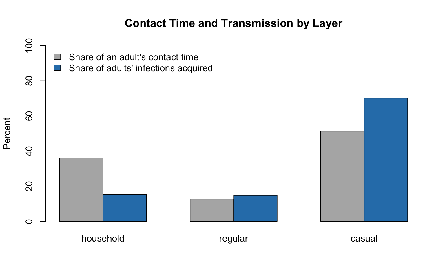

Figure 1: Share of an adult’s daily contact time spent on each layer (gray; McCreesh and White 2018) and share of adults’ infections acquired on each layer in the baseline structure over the last 20 years of burn-in (blue), mean of simulations.

Households hold 36% of an adult’s contact time, but adults acquired 15% of their infections at home and 70% from casual contacts, which hold 51% of their time. Two features of the network produce the gap, and neither is a parameter that says households transmit less:

1. Saturation of persistent ties. A person with TB meets the same few co-residents month after month. Once they are infected, and in this setting many already were before the case began, further contact produces little new infection: reinfection of someone with prior infection is 79% less likely to succeed, and someone in early latency or with TB cannot be infected again. An edge can transmit only once, and a household edge stays the same edge for years; casual contact brings new people every month.
2. Overdispersion. With inf.k = 0.15, about 40% of cases have less than 1% of the average infectiousness and transmit almost nothing anywhere, while a few are many times more infectious than average. A highly infectious case infects most of its household within months, and the rest of its transmission goes to its regular and casual contacts.

The regular layer, persistent but open (a coworker’s own contacts are mostly not the case’s), gives adults 15% of their infections for 13% of their contact time.

The persistence of ties

knitr::kable(struct_tbl,
             col.names = c("Structure", "Incidence", "Change from baseline (%)",
                           "Children", "Adults", "Household (%)", "Regular (%)",
                           "Casual (%)", "Reinfections (%)"),
             caption = "TB incidence per 100,000 per year (all ages, children, adults), the percent change in all-ages incidence from the baseline, the share of all infections transmitted on each layer, and the share of infections that were reinfections, over the last 20 years of burn-in; mean (95% Monte Carlo interval). In household_redrawn the household column is the redrawn layer that carries household contact time.")

Table 2: TB incidence per 100,000 per year (all ages, children, adults), the percent change in all-ages incidence from the baseline, the share of all infections transmitted on each layer, and the share of infections that were reinfections, over the last 20 years of burn-in; mean (95% Monte Carlo interval). In household_redrawn the household column is the redrawn layer that carries household contact time.

Structure	Incidence	Change from baseline (%)	Children	Adults	Household (%)	Regular (%)	Casual (%)	Reinfections (%)
baseline	450 (368, 532)	reference	311 (253, 370)	494 (404, 585)	20.1 (19.2, 21.0)	14.1 (13.8, 14.4)	65.8 (64.9, 66.8)	61.8 (56.7, 67.0)
regular_redrawn	564 (452, 675)	25.2 (-3.3, 53.7)	405 (319, 492)	614 (494, 735)	19.1 (18.5, 19.8)	21.3 (21.0, 21.7)	59.5 (58.9, 60.2)	68.1 (65.4, 70.7)
household_redrawn	683 (550, 816)	51.8 (19.5, 84.1)	637 (521, 752)	698 (558, 838)	38.2 (38.0, 38.4)	11.2 (11.1, 11.4)	50.6 (50.3, 50.9)	74.2 (70.4, 78.0)

inc_st <- lapply(burn, annual, vars = inc_all, rows = 2:burnin)
par(mfrow = c(1, 1), mar = c(4, 4.5, 2, 1))
plot(NA, xlim = c(1, length(inc_st$baseline)),
     ylim = c(0, max(unlist(inc_st)) * 1.05),
     xlab = "Year of burn-in", ylab = "TB incidence per 100,000 per year",
     main = "Incidence by Contact Structure")
for (s in names(inc_st)) lines(inc_st[[s]], col = cols_st[s], lwd = 2)
legend("topright", legend = names(inc_st), col = cols_st, lwd = 2, bty = "n")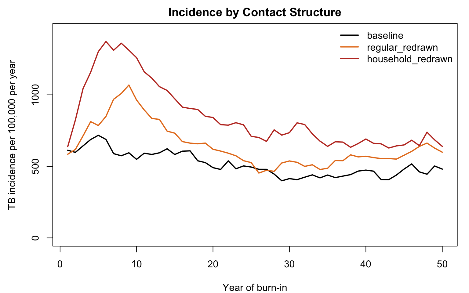

Figure 2: TB incidence per 100,000 per year over the 50-year burn-in, by contact structure, mean of simulations.

With the same contact time and the same per-hour risk, redrawing regular contacts every month changed incidence by 25.2% (95% Monte Carlo interval -3.3 to 53.7), and spreading household contact time over new partners every month changed it by 51.8% (95% Monte Carlo interval 19.5 to 84.1). In the redrawn-household structure, the layer that carries household contact time transmitted 38% of all infections, close to the share of contact time it holds: once the same hours are spent with new people each month, the gap between contact time and transmission all but disappears. Reinfections also made up more of all infections, 74% rather than 62%, because with more transmission more of the population has been infected before.

The early decades of each curve are the adjustment of the latent pool from the starting states, which overshoots before settling. The comparison uses the last 20 years, over which incidence changed from the first half to the second by +17% in the baseline, +15% with regular contacts redrawn, and +5% with household contact redrawn. Where that drift is large, the structure’s difference from the baseline is uncertain in timing as well as size, and a longer burn-in would settle it.

The redrawn structures are what a well-mixed model assumes about contact. A compartmental model that allocated transmission in proportion to contact time would behave like household_redrawn: fitted to the same incidence, it would need a lower per-contact risk, and it would place about 36% of adults’ infections in households rather than the 15% the network produces. The household share is the quantity on which the value of a household program depends, which Part 2 examines.

Part 2: Household Investigation versus Community-wide Screening

The second experiment resumes each baseline simulation from the end of its burn-in and runs each program for 10 years. Every scenario resumes simulation s from the same burn-in state s, so differences between scenarios are paired by simulation; their random numbers diverge as soon as a program draws its first one.

Scenario	Program
none	passive case finding only
hhci_screen	household contact investigation for every newly diagnosed person: contacts are screened for active TB, with no TPT
hhci_u5	the same investigation, with TPT offered to contacts under 5
hhci_all	the same investigation, with TPT offered to contacts of all ages
acf	community-wide screening: an annual round that tests 42% of people 15 and older, with no TPT
random	the hhci_all package (screening plus TPT for all ages) given to people chosen at random, at the average monthly rate at which hhci_all screened contacts

The three household arms screen the same way and differ only in who is offered TPT, so comparing them isolates the preventive therapy. The random arm is the equal-effort comparator: it screens and treats as many people as hhci_all, so the difference between the two is the value of choosing whom to screen through the household link.

scenarios.df <- data.frame(
  .scenario.id = c("none", "hhci_screen", "hhci_u5", "hhci_all", "acf"),
  .at = 1,
  hhci = c(0, 1, 1, 1, 0),
  tpt.age.max = c(Inf, 0, 5, Inf, Inf),
  acf = c(0, 0, 0, 0, 1)
)
scenarios.list <- create_scenario_list(scenarios.df)

1burnin_sims <- lapply(seq_len(nsims), function(s) get_sims(burn$baseline, s))
resume <- make_control(burnin + horizon, structures$baseline$tergm,
                       start = burnin + 1, sims = 1, cores = 1)
run_scenario <- function(scn) {
2  param_scn <- use_scenario(param_base, scn)
  runs <- future.apply::future_lapply(burnin_sims, function(x) {
    netsim(x, param_scn, init, resume)
3  }, future.seed = 202)
4  Reduce(merge, runs)
}
future::plan("multisession", workers = ncores)
sims <- list()
for (scn in scenarios.list) {
  cat("Scenario:", scn$id, "\n")
  sims[[scn$id]] <- run_scenario(scn)
}

# Equal-effort comparator: screen people chosen at random, with the same
# package, at the average monthly rate at which household investigation
# screened contacts in the hhci_all scenario.
rows_h <- burnin + seq_len(horizon)
hh_screened <- mean(epi_sum(sims$hhci_all, "hh.screened", rows_h)) / horizon
pop_h <- mean(epi_sum(sims$hhci_all, c("num.child", "num.adult"), rows_h)) / horizon
random.rate <- hh_screened / pop_h
rnd <- create_scenario_list(data.frame(.scenario.id = "random", .at = 1,
                                       random.rate = random.rate,
                                       tpt.age.max = Inf))
sims$random <- run_scenario(rnd[[1]])
future::plan("sequential")

1

A resumed run restarts every one of its simulations from the first simulation of the netsim object it is given, so passing burn$baseline itself would start all 10 simulations of every scenario from the same state. get_sims() extracts each burn-in simulation, with its run state, as a netsim object of its own, keeping the burn-in’s step numbers, so the time attributes (infTime, dxTime, hhcTime) need no adjustment.

2

The resumed run takes its parameters from param alone, which must hold every parameter of the model; use_scenario() returns the base set with the scenario’s values.

3

future_lapply() runs the single-simulation resumptions in parallel, as netsim() itself does when ncores is above 1, and a fixed future.seed gives burn-in simulation s the same random number stream in every scenario.

4

merge() combines netsim objects with the same parameters and controls, so simulation s of each scenario is the run from burn-in simulation s.

Scenario: none 
Scenario: hhci_screen 
Scenario: hhci_u5 
Scenario: hhci_all 
Scenario: acf 

Population impact

scn_ids <- names(sims)
labels <- c(none = "Passive case finding only",
            hhci_screen = "Household investigation, no TPT",
            hhci_u5 = "Household investigation, TPT under 5",
            hhci_all = "Household investigation, TPT all ages",
            acf = "Community-wide screening of adults",
            random = "Random screening, equal effort")
bands <- c("u5", "5to14", "adult")

# Per-simulation outcomes over the horizon. The contact outcomes use years 3
# to 10: TB onsets within 24 months of being identified as a household
# contact of a newly diagnosed case, and the contacts identified, in the
# same months. In a steady state their ratio is the two-year risk.
rows_c <- burnin + (min(24, horizon - 1) + 1):horizon
rows_y4 <- burnin + (min(36, horizon - 1) + 1):min(48, horizon)  # year 4
outcomes <- function(sim) {
  pop <- epi_mean(sim, c("num.child", "num.adult"), rows_h)
  list(
    pop = pop,
    inc = epi_sum(sim, c(inc_vars("child"), inc_vars("adult")), rows_h),
    inc_child = epi_sum(sim, inc_vars("child"), rows_h),
    deaths = epi_sum(sim, c("tbdeath.child", "tbdeath.adult"), rows_h),
    screened = epi_sum(sim, c("hh.screened", "rnd.screened", "acf.screened"), rows_h),
    found = epi_sum(sim, c("hh.found", "rnd.found", "acf.found"), rows_h),
    tpt = epi_sum(sim, "tpt.completed", rows_h),
    prev_adult_y4 = epi_mean(sim, "i.num.adult", rows_y4),
    contacts_u5 = epi_sum(sim, "hhc.n.u5", rows_c),
    contacts_5p = epi_sum(sim, c("hhc.n.5to14", "hhc.n.adult"), rows_c),
    contact_tb_u5 = epi_sum(sim, "hhc.inc.u5", rows_c),
    contact_tb_5p = epi_sum(sim, c("hhc.inc.5to14", "hhc.inc.adult"), rows_c),
    tpt_c = epi_sum(sim, "tpt.completed", rows_c)
  )
}
oc <- lapply(sims, outcomes)
per100k <- function(x, pop) 1e5 * x / pop

# Population impact: differences from passive case finding, paired by
# simulation (every scenario resumes simulation s from the same burn-in
# state s), with 95% Monte Carlo intervals.
impact_tbl <- data.frame(
  scenario = labels[scn_ids],
  incidence = sapply(scn_ids, function(s)
    fmt(mc(per100k_yr(oc[[s]]$inc, oc[[s]]$pop, rows_h)))),
  tb_averted = sapply(scn_ids, function(s)
    fmt(mc(per100k(oc$none$inc - oc[[s]]$inc, oc$none$pop)))),
  pct_averted = sapply(scn_ids, function(s)
    fmt(mc(100 * (oc$none$inc - oc[[s]]$inc) / mean(oc$none$inc)), 1)),
  child_tb_averted = sapply(scn_ids, function(s)
    fmt(mc(per100k(oc$none$inc_child - oc[[s]]$inc_child, oc$none$pop)))),
  deaths_averted = sapply(scn_ids, function(s)
    fmt(mc(per100k(oc$none$deaths - oc[[s]]$deaths, oc$none$pop)))),
  row.names = NULL
)
knitr::kable(impact_tbl,
             col.names = c("Scenario", "Incidence per 100,000 per year",
                           "TB averted per 100,000", "TB averted (%)",
                           "Child TB averted per 100,000", "TB deaths averted per 100,000"),
             caption = "Population impact over 10 years: incidence, and TB cases, child TB cases, and TB deaths averted relative to passive case finding, paired by simulation; mean (95% Monte Carlo interval)")

Table 3: Population impact over 10 years: incidence, and TB cases, child TB cases, and TB deaths averted relative to passive case finding, paired by simulation; mean (95% Monte Carlo interval)

Scenario	Incidence per 100,000 per year	TB averted per 100,000	TB averted (%)	Child TB averted per 100,000	TB deaths averted per 100,000
Passive case finding only	474 (390, 558)	0 (0, 0)	0.0 (0.0, 0.0)	0 (0, 0)	0 (0, 0)
Household investigation, no TPT	471 (385, 556)	25 (-1042, 1092)	0.4 (-22.2, 23.0)	9 (-176, 194)	34 (-81, 149)
Household investigation, TPT under 5	471 (396, 545)	26 (-813, 866)	0.5 (-17.3, 18.2)	23 (-137, 183)	30 (-65, 125)
Household investigation, TPT all ages	392 (302, 483)	813 (209, 1418)	17.1 (4.3, 29.9)	180 (87, 273)	97 (4, 191)
Community-wide screening of adults	334 (259, 409)	1393 (388, 2397)	29.4 (8.2, 50.5)	263 (99, 427)	213 (114, 313)
Random screening, equal effort	467 (395, 539)	60 (-760, 880)	1.2 (-16.1, 18.5)	-38 (-172, 97)	8 (-97, 113)

# Community-wide screening against ACT3: adult prevalence of active TB in
# year 4 (after three annual rounds), relative to passive case finding
acf_prev_ratio <- mc(oc$acf$prev_adult_y4 / oc$none$prev_adult_y4)
fmt(acf_prev_ratio, 2)

[1] "0.69 (0.51, 0.87)"

cols_scn <- c(none = "black", hhci_screen = "#a6bddb", hhci_u5 = "#74a9cf",
              hhci_all = "#0570b0", acf = "#d95f0e", random = "#756bb1")
rows_ctx <- max(2, burnin - 59):(burnin + horizon)
inc_scn <- lapply(sims, annual, vars = inc_all, rows = rows_ctx)
yrs <- seq_along(inc_scn$none) - ceiling((burnin - min(rows_ctx) + 1) / 12)
plot(NA, xlim = range(yrs), ylim = c(0, max(unlist(inc_scn)) * 1.05),
     xlab = "Years since programs started", ylab = "TB incidence per 100,000 per year",
     main = "Incidence by Intervention")
abline(v = 0.5, lty = 3)
for (s in names(inc_scn)) lines(yrs, inc_scn[[s]], col = cols_scn[s], lwd = 2)
legend("bottomleft", legend = labels[names(inc_scn)], col = cols_scn[names(inc_scn)],
       lwd = 2, bty = "n", cex = 0.8)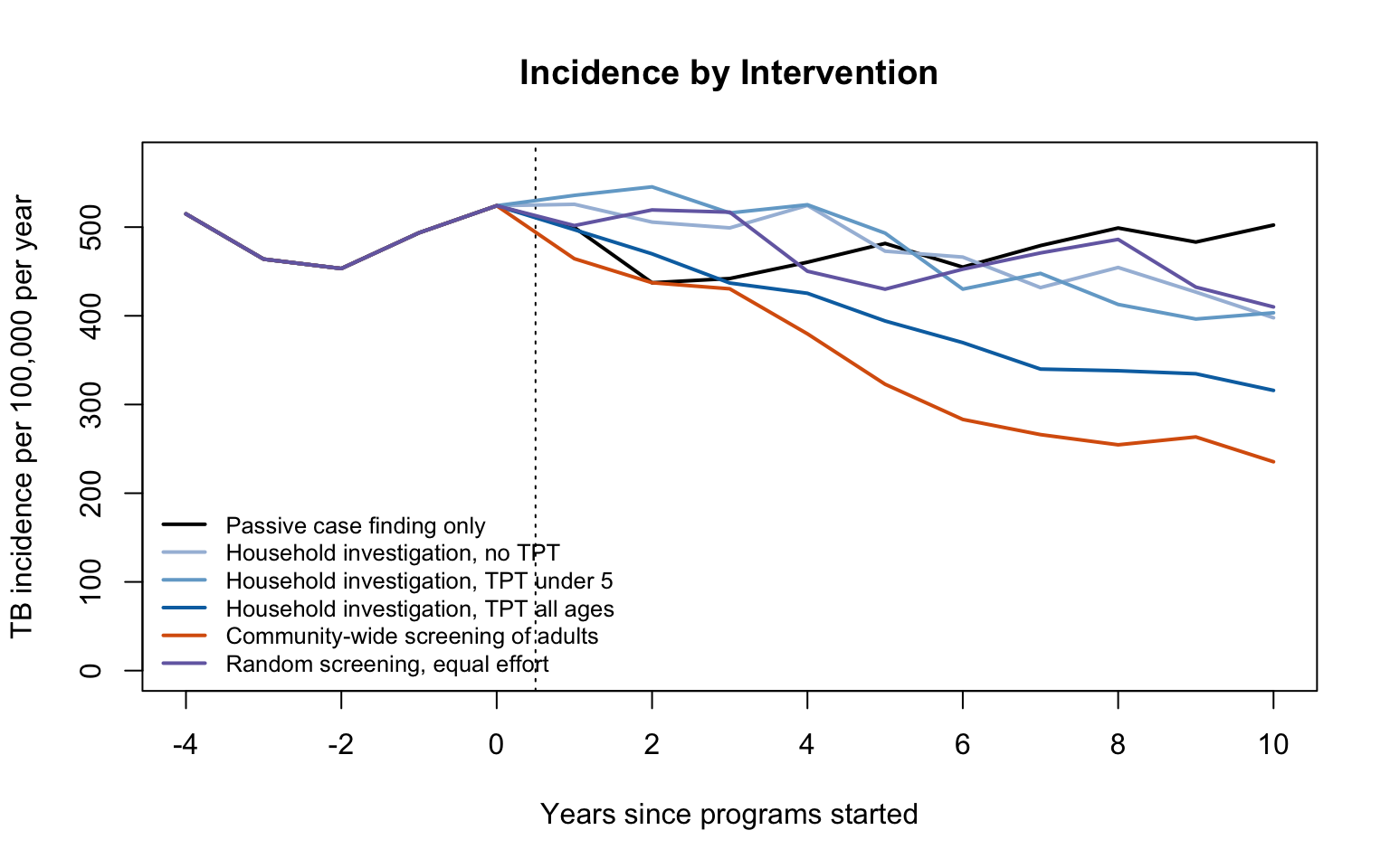

Figure 3: TB incidence per 100,000 per year by scenario, for the last five years of the burn-in and the ten years of the programs, mean of simulations.

scn_int <- setdiff(scn_ids, "none")
short <- c(hhci_screen = "Household, no TPT", hhci_u5 = "Household, TPT <5",
           hhci_all = "Household, TPT all", acf = "Community-wide",
           random = "Random, equal effort")
diffs <- matrix(sapply(scn_int, function(s) per100k(oc$none$inc - oc[[s]]$inc, oc$none$pop)),
                ncol = length(scn_int), dimnames = list(NULL, scn_int))
par(mfrow = c(1, 1), mar = c(9, 5, 3, 1))
plot(NA, xlim = c(0.5, length(scn_int) + 0.5), ylim = range(c(0, diffs)) * 1.1,
     xaxt = "n", xlab = "", ylab = "TB averted per 100,000 over 10 years",
     main = "Population Impact")
abline(h = 0, lty = 3)
for (j in seq_along(scn_int)) {
  points(j + runif(nrow(diffs), -0.15, 0.15), diffs[, j], pch = 19,
         col = adjustcolor(cols_scn[scn_int[j]], 0.6))
  ci <- mc(diffs[, j])
  segments(j - 0.25, ci["est"], j + 0.25, ci["est"], lwd = 3)
  if (!is.na(ci["lo"])) arrows(j, ci["lo"], j, ci["hi"], angle = 90, code = 3, length = 0.05)
}
axis(1, at = seq_along(scn_int), labels = short[scn_int], las = 2, cex.axis = 0.85)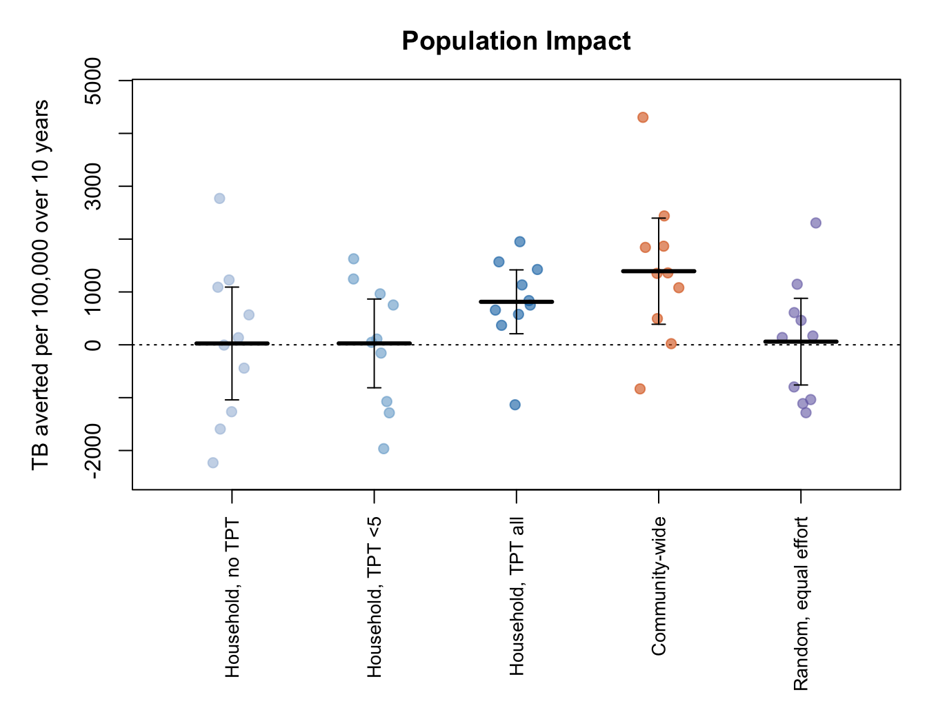

Figure 4: TB cases averted per 100,000 over 10 years relative to passive case finding, one point per simulation, with the mean (bar) and 95% Monte Carlo interval.

Community-wide screening of adults averted 29.4% (95% Monte Carlo interval 8.2 to 50.5) of incident TB over 10 years. ACT3 measured prevalence rather than incidence: after three annual rounds, adult prevalence in the screened communities was 0.56 times that in the control communities (Marks et al. 2019), and the model’s ratio of adult prevalence in year 4 to that under passive case finding was 0.69 (95% Monte Carlo interval 0.51 to 0.87). Household investigation averted 0.4% (95% Monte Carlo interval -22.2 to 23.0) without TPT, 0.5% (95% Monte Carlo interval -17.3 to 18.2) with TPT for contacts under 5, and 17.1% (95% Monte Carlo interval 4.3 to 29.9) with TPT for contacts of all ages; the random arm, with the same effort and the same package as the last, averted 1.2% (95% Monte Carlo interval -16.1 to 18.5). With 10 simulations, one of the household arms has an effect distinguishable from zero, and the random arm’s effect is not.

The spread of the points in the figure is the reason to read these rows with their intervals. This model sits where small changes in transmission move incidence a lot: in Part 1, rearranging the same contact hours changed incidence by as much as 52%, and each active case a program finds early averts further cases over the rest of the decade (next section). The population effects of programs that find a few percent of cases early therefore vary widely between simulations, even though every scenario starts from the same state, and 10 simulations do not pin them down. Across this run and two others with different seeds, community-wide screening averted 29 to 44% of incident TB, with an interval that always excluded zero; household investigation with TPT for all ages averted 9 to 19%, distinguishable from zero in one of the three; and the other two household arms (0 to 11%) and the random arm (-4 to 2%) never were. Prior models place the population effect of household contact tracing at 4 to 27% over five years (Kasaie et al. 2014; Havumaki et al. 2023).

Yield and the direct protection of contacts

The programs’ own outcomes are measured on the people they reach and vary much less between simulations than population incidence.

# Program yield. Screenings count every screen, so a person screened in
# several community rounds counts several times. TB averted per case found
# divides the mean cases averted by the mean cases found by the program.
program_tbl <- data.frame(
  scenario = labels[scn_ids],
  screenings = sapply(scn_ids, function(s) round(mean(per100k(oc[[s]]$screened, oc[[s]]$pop)))),
  found = sapply(scn_ids, function(s) round(mean(per100k(oc[[s]]$found, oc[[s]]$pop)))),
  found_per_1000 = sapply(scn_ids, function(s)
    if (sum(oc[[s]]$screened) == 0) NA else
      round(1000 * sum(oc[[s]]$found) / sum(oc[[s]]$screened), 1)),
  tpt_completed = sapply(scn_ids, function(s) round(mean(per100k(oc[[s]]$tpt, oc[[s]]$pop)))),
  averted_per_found = sapply(scn_ids, function(s)
    if (sum(oc[[s]]$found) == 0) NA else
      round(sum(oc$none$inc - oc[[s]]$inc) / sum(oc[[s]]$found), 1)),
  row.names = NULL
)
knitr::kable(program_tbl,
             col.names = c("Scenario", "Screenings per 100,000", "Active TB found per 100,000",
                           "Found per 1,000 screenings", "TPT courses completed per 100,000",
                           "TB averted per case found"),
             caption = "Program yield over 10 years per 100,000 population, pooled over simulations. Screenings count every screen, so a person screened in several community rounds counts several times.")

Table 4: Program yield over 10 years per 100,000 population, pooled over simulations. Screenings count every screen, so a person screened in several community rounds counts several times.

Scenario	Screenings per 100,000	Active TB found per 100,000	Found per 1,000 screenings	TPT courses completed per 100,000	TB averted per case found
Passive case finding only	0	0	NA	0	NA
Household investigation, no TPT	9603	250	26.0	0	0.1
Household investigation, TPT under 5	9522	244	25.6	666	0.1
Household investigation, TPT all ages	8178	192	23.5	5425	4.2
Community-wide screening of adults	318760	897	2.8	0	1.5
Random screening, equal effort	8224	30	3.6	5582	1.9

yield <- program_tbl$found_per_1000[match(scn_int, scn_ids)]
bp2 <- barplot(yield, names.arg = short[scn_int], las = 2, col = cols_scn[scn_int],
               cex.names = 0.85, ylim = c(0, max(yield, na.rm = TRUE) * 1.2),
               ylab = "Active TB found per 1,000 screened", main = "Yield of Screening")
text(bp2, yield + max(yield, na.rm = TRUE) * 0.05, yield, cex = 0.9)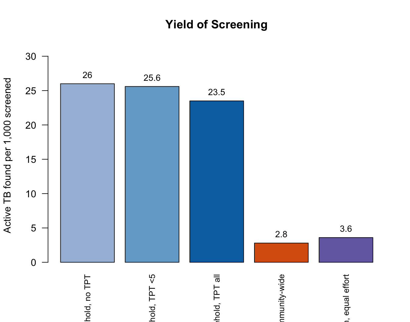

Figure 5: Active TB found per 1,000 screenings by each program over 10 years, pooled over simulations.

Household investigation found active TB in 23.5 of every 1,000 contacts screened, 7 times the yield of the same package given to people chosen at random and 8 times the yield of community-wide rounds, which made 39 times as many screenings. Each case the community-wide program found early averted, on average, 1.5 further cases over the decade, the leverage that makes early diagnosis worth more than the cases it finds; the same ratio for the household arm without TPT, 0.1, inherits the noise of that arm’s population effect.

# The direct effect of TPT on household contacts. The three household arms
# screen the same way and differ only in who is offered TPT, so contacts
# under 5 are compared between no TPT and TPT under 5, and contacts 5 and
# older between TPT under 5 and TPT for all ages. Risks are TB onsets within
# 24 months per 1,000 contacts identified, pooled over simulations.
risk <- function(o, grp) 1000 * sum(o[[paste0("contact_tb_", grp)]]) /
  sum(o[[paste0("contacts_", grp)]])
tpt_effect <- function(without, with, grp, courses) {
  r0 <- risk(oc[[without]], grp)
  r1 <- risk(oc[[with]], grp)
  averted <- (r0 - r1) / 1000 * sum(oc[[with]][[paste0("contacts_", grp)]])
  c(risk_without = round(r0, 1), risk_with = round(r1, 1),
    pct_reduction = round(100 * (r0 - r1) / r0),
    courses_per_case_averted = if (isTRUE(averted > 0)) round(courses / averted) else NA)
}
tpt_tbl <- rbind(
  "Contacts under 5" = tpt_effect("hhci_screen", "hhci_u5", "u5",
                                  sum(oc$hhci_u5$tpt_c)),
  "Contacts 5 and older" = tpt_effect("hhci_u5", "hhci_all", "5p",
                                      sum(oc$hhci_all$tpt_c) - sum(oc$hhci_u5$tpt_c))
)
knitr::kable(tpt_tbl,
             col.names = c("TB within 2 years per 1,000, without TPT", "With TPT",
                           "Reduction (%)", "Completed TPT courses per case averted"),
             caption = "TB onsets within two years among household contacts identified in years 3 to 10, in the household arm without TPT for that age group and the arm with it, pooled over simulations")

Table 5: TB onsets within two years among household contacts identified in years 3 to 10, in the household arm without TPT for that age group and the arm with it, pooled over simulations

	TB within 2 years per 1,000, without TPT	With TPT	Reduction (%)	Completed TPT courses per case averted
Contacts under 5	38.4	29.8	22	44
Contacts 5 and older	27.4	17.7	36	36

Because the household arms screen the same way, the differences in this table are the effect of the preventive therapy itself. Comparing any program with passive case finding would also credit it with its effect on transmission, which lowers every contact’s risk: the community-wide arm, which gives no TPT and investigates no households, lowers household contacts’ risk too. TPT reduced the two-year risk of TB among contacts under 5 by 22%, at 44 completed courses per case averted, and among contacts 5 and older by 36%, at 36 courses per case averted. Contacts under 5 are few, about 2,700 identified in years 3 to 10 over all 10 simulations with 104 TB onsets in the arm without TPT, so their estimate is the noisy one: across this run and two others with different seeds it ranged from -9% to 28%, against 26 to 36% for contacts 5 and older. In Lima, preventive therapy for household contacts with a positive skin test prevented about 30 cases per 1,000 courses (Zelner et al. 2018); the model offers TPT without testing, so part of every course goes to a contact who is not infected. Extending TPT from children under 5 to contacts of all ages added about 4,759 completed courses per 100,000 over the decade, which at that rate prevents about 132 cases per 100,000 directly, 2.8% of incident TB.

# The most a household program could prevent directly: the share of all
# incident TB, under passive case finding, that occurs in people identified
# as a household contact in the previous 24 months
contact_share <- 100 * (oc$none$contact_tb_u5 + oc$none$contact_tb_5p) /
  epi_sum(sims$none, c(inc_vars("child"), inc_vars("adult")), rows_c)
fmt(mc(contact_share), 1)

[1] "10.5 (8.9, 12.1)"

Under passive case finding, 10.5% of all incident TB occurred in people who had been household contacts of a newly diagnosed case in the previous two years. That is the most a household program could prevent directly, even with complete coverage and perfect TPT. Whatever it achieves beyond that comes indirectly, by finding infectious people earlier and so shortening the time in which they transmit, most of it outside the household. This is the network’s account of why household contact investigation is efficient for the people it reaches but limited in what it can do directly for the population. In the ZAMSTAR trial in Zambia and South Africa, communities randomized to a household-based intervention had 18% lower TB prevalence, with a confidence interval that included no effect (prevalence ratio 0.82, 95% CI 0.64 to 1.04; Ayles et al. 2013).

Between-simulation variability

cv <- sapply(st, function(x) sd(x$inc) / mean(x$inc))
round(cv, 2)

         baseline   regular_redrawn household_redrawn 
             0.25              0.28              0.27 

The coefficient of variation of incidence across the 10 baseline simulations, each averaged over 20 years, is 0.25. Two features of the model produce this much variation: transmission is concentrated in a few highly infectious cases, and the population of 20,000 has on average only 77 people with undiagnosed active TB at a time. More simulations narrow the intervals in proportion to the square root of their number, and a larger population narrows them further, at a cost in run time that grows with both. Resuming each burn-in state several times with different random numbers is a cheaper way to tighten the Part 2 comparisons, since most of their noise arises after the programs start.

Next Steps

• HIV. Add a fixed or dynamic HIV attribute that multiplies progression, reactivation, and TB mortality, with antiretroviral therapy reducing them. This is what a Southern African TB model needs first, and it would also make household clustering of HIV, and so of TB risk, a network question.
• Subclinical TB. Split active TB into subclinical and clinical states with transitions both ways, so that screening finds people passive case finding never would. The community-wide arm would gain the most.
• Sex and heterogeneous contact. Give adult men more casual contact time, and let casual degree vary between people rather than only between age groups; the non-repeated contacts in the Western Cape survey had a variance twelve times their mean.
• Where contact happens. Weight contact-hours by the ventilation of the setting (households, transport, workplaces, clinics), so that per-hour risk differs between layers. Model conclusions about the household share are sensitive to the ratio of per-hour risk in public places to that at home.
• Contact investigation beyond the household. Turning on the cumulative edgelist (cumulative.edgelist = TRUE in control.net(), with truncate.el.cuml at least as long as the lookback) would record the regular layer’s partnerships, so that each index case’s regular contacts over a lookback window could be investigated with get_partners(); see the contact tracing example.
• More casual edges. Raise the casual layer’s degree and lower its hours per edge toward the hundreds of brief contacts a month in the Western Cape survey, with the TERGM chain lengthened in proportion, and see how far the household share falls.
• More replicates for Part 2. Resume each burn-in state several times with different random numbers to tighten the program comparisons, whose noise arises mostly after the programs start.
• TPT with a duration. Hold contacts in a treatment state for the three months of 3HP, during which recently infected contacts can still progress, and add an effect on reinfection during the course.
• A prevention-of-disease vaccine. Rothman et al. (2026) targeted a vaccine by clinical risk group in the United States; in this network it could be targeted by exposure, to household contacts of newly diagnosed people, and compared with vaccinating the same number of people at random.
• Matched-incidence comparisons. Part 1 compares contact structures at fixed per-hour risk. Tuning beta separately for each structure to the same incidence, and then running the Part 2 programs in each, asks the other half of the question: how much the value of household targeting depends on how much transmission a model places in households.

References

TB transmission in households and the community:

• McCreesh N, White RG. (2018). An explanation for the low proportion of tuberculosis that results from transmission between household and known social contacts. Sci Rep 8:5382. https://doi.org/10.1038/s41598-018-23797-2
• Verver S, Warren RM, Munch Z, et al. (2004). Proportion of tuberculosis transmission that takes place in households in a high-incidence area. Lancet 363(9404):212-214. https://doi.org/10.1016/S0140-6736(03)15332-9
• Glynn JR, Guerra-Assunção JA, Houben RMGJ, et al. (2015). Whole genome sequencing shows a low proportion of tuberculosis disease is attributable to known close contacts in rural Malawi. PLoS One 10(7):e0132840. https://doi.org/10.1371/journal.pone.0132840
• Middelkoop K, Mathema B, Myer L, et al. (2015). Transmission of tuberculosis in a South African community with a high prevalence of HIV infection. J Infect Dis 211(1):53-61. https://doi.org/10.1093/infdis/jiu403
• Martinez L, Shen Y, Mupere E, Kizza A, Hill PC, Whalen CC. (2017). Transmission of Mycobacterium tuberculosis in households and the community: a systematic review and meta-analysis. Am J Epidemiol 185(12):1327-1339. https://doi.org/10.1093/aje/kwx025
• Martinez L, Lo NC, Cords O, et al. (2019). Paediatric tuberculosis transmission outside the household: challenging historical paradigms to inform future public health strategies. Lancet Respir Med 7(6):544-552. https://doi.org/10.1016/S2213-2600(19)30137-7
• Zelner JL, Murray MB, Becerra MC, et al. (2014). Age-specific risks of tuberculosis infection from household and community exposures and opportunities for interventions in a high-burden setting. Am J Epidemiol 180(8):853-861. https://doi.org/10.1093/aje/kwu192
• Andrews JR, Morrow C, Walensky RP, Wood R. (2014). Integrating social contact and environmental data in evaluating tuberculosis transmission in a South African township. J Infect Dis 210(4):597-603. https://doi.org/10.1093/infdis/jiu138

Household contacts and contact investigation:

• Fox GJ, Barry SE, Britton WJ, Marks GB. (2013). Contact investigation for tuberculosis: a systematic review and meta-analysis. Eur Respir J 41(1):140-156. https://doi.org/10.1183/09031936.00070812
• Velen K, Shingde RV, Ho J, Fox GJ. (2021). The effectiveness of contact investigation among contacts of tuberculosis patients: a systematic review and meta-analysis. Eur Respir J 58(6):2100266. https://doi.org/10.1183/13993003.00266-2021
• Martinez L, Cords O, Horsburgh CR, et al. (2020). The risk of tuberculosis in children after close exposure: a systematic review and individual-participant meta-analysis. Lancet 395(10228):973-984. https://doi.org/10.1016/S0140-6736(20)30166-5
• Zelner J, Murray M, Becerra M, et al. (2018). Protective effects of household-based TB interventions are robust to neighbourhood-level variation in exposure risk in Lima, Peru: a model-based analysis. Int J Epidemiol 47(1):185-192. https://doi.org/10.1093/ije/dyx171
• Kasaie P, Andrews JR, Kelton WD, Dowdy DW. (2014). Timing of tuberculosis transmission and the impact of household contact tracing: an agent-based simulation model. Am J Respir Crit Care Med 189(7):845-852. https://doi.org/10.1164/rccm.201310-1846OC
• Havumaki J, Cohen T, Zhai C, et al. (2021). Protective impacts of household-based tuberculosis contact tracing are robust across endemic incidence levels and community contact patterns. PLoS Comput Biol 17(2):e1008713. https://doi.org/10.1371/journal.pcbi.1008713
• Havumaki J, Warren JL, Zelner J, et al. (2023). Spatially-targeted tuberculosis screening has limited impact beyond household contact tracing in Lima, Peru: a model-based analysis. PLoS One 18(10):e0293519. https://doi.org/10.1371/journal.pone.0293519
• Marks GB, Nguyen NV, Nguyen PTB, et al. (2019). Community-wide screening for tuberculosis in a high-prevalence setting. N Engl J Med 381(14):1347-1357. https://doi.org/10.1056/NEJMoa1902129
• Ayles H, Muyoyeta M, Du Toit E, et al. (2013). Effect of household and community interventions on the burden of tuberculosis in southern Africa: the ZAMSTAR community-randomised trial. Lancet 382(9899):1183-1194. https://doi.org/10.1016/S0140-6736(13)61131-9
• Sterling TR, Villarino ME, Borisov AS, et al. (2011). Three months of rifapentine and isoniazid for latent tuberculosis infection. N Engl J Med 365(23):2155-2166. https://doi.org/10.1056/NEJMoa1104875
• Villarino ME, Scott NA, Weis SE, et al. (2015). Treatment for preventing tuberculosis in children and adolescents: a randomized clinical trial of a 3-month, 12-dose regimen of a combination of rifapentine and isoniazid. JAMA Pediatr 169(3):247-255. https://doi.org/10.1001/jamapediatrics.2014.3158
• Churchyard GJ, Fielding KL, Lewis JJ, et al. (2014). A trial of mass isoniazid preventive therapy for tuberculosis control. N Engl J Med 370(4):301-310. https://doi.org/10.1056/NEJMoa1214289

Natural history:

• Rothman JE, Castro KG, Lopman BA, Gandhi NR, Nelson KN. (2026). Targeted tuberculosis vaccination strategies in the United States: a modeling study. Vaccine 92:129174. https://doi.org/10.1016/j.vaccine.2026.129174
• Trauer JM, Moyo N, Tay EL, et al. (2016). Risk of active tuberculosis in the five years following infection . . . 15%? Chest 149(2):516-525. https://doi.org/10.1016/j.chest.2015.11.017
• Ragonnet R, Trauer JM, Scott N, Meehan MT, Denholm JT, McBryde ES. (2017). Optimally capturing latency dynamics in models of tuberculosis transmission. Epidemics 21:39-47. https://doi.org/10.1016/j.epidem.2017.06.002
• Vynnycky E, Fine PEM. (1997). The natural history of tuberculosis: the implications of age-dependent risks of disease and the role of reinfection. Epidemiol Infect 119(2):183-201. https://doi.org/10.1017/s0950268897007917
• Marais BJ, Gie RP, Schaaf HS, et al. (2004). The natural history of childhood intra-thoracic tuberculosis: a critical review of literature from the pre-chemotherapy era. Int J Tuberc Lung Dis 8(4):392-402. PMID 15141729.
• Andrews JR, Noubary F, Walensky RP, Cerda R, Losina E, Horsburgh CR. (2012). Risk of progression to active tuberculosis following reinfection with Mycobacterium tuberculosis. Clin Infect Dis 54(6):784-791. https://doi.org/10.1093/cid/cir951
• Verver S, Warren RM, Beyers N, et al. (2005). Rate of reinfection tuberculosis after successful treatment is higher than rate of new tuberculosis. Am J Respir Crit Care Med 171(12):1430-1435. https://doi.org/10.1164/rccm.200409-1200OC
• Emery JC, Richards AS, Dale KD, et al. (2021). Self-clearance of Mycobacterium tuberculosis infection: implications for lifetime risk and population at-risk of tuberculosis disease. Proc R Soc B 288(1943):20201635. https://doi.org/10.1098/rspb.2020.1635
• Tiemersma EW, van der Werf MJ, Borgdorff MW, Williams BG, Nagelkerke NJD. (2011). Natural history of tuberculosis: duration and fatality of untreated pulmonary tuberculosis in HIV negative patients: a systematic review. PLoS One 6(4):e17601. https://doi.org/10.1371/journal.pone.0017601
• Jenkins HE, Yuen CM, Rodriguez CA, et al. (2017). Mortality in children diagnosed with tuberculosis: a systematic review and meta-analysis. Lancet Infect Dis 17(3):285-295. https://doi.org/10.1016/S1473-3099(16)30474-1
• Vega V, Rodríguez S, Van der Stuyft P, Seas C, Otero L. (2021). Recurrent TB: a systematic review and meta-analysis of the incidence rates and the proportions of relapses and reinfections. Thorax 76(5):494-502. https://doi.org/10.1136/thoraxjnl-2020-215449

Network and household models of TB:

• Aparicio JP, Capurro AF, Castillo-Chavez C. (2000). Transmission and dynamics of tuberculosis on generalized households. J Theor Biol 206(3):327-341. https://doi.org/10.1006/jtbi.2000.2129
• Cohen T, Colijn C, Finklea B, Murray M. (2007). Exogenous re-infection and the dynamics of tuberculosis epidemics: local effects in a network model of transmission. J R Soc Interface 4(14):523-531. https://doi.org/10.1098/rsif.2006.0193
• Pando C, Hazel A, Tsang LY, et al. (2023). A social network analysis model approach to understand tuberculosis transmission in remote rural Madagascar. BMC Public Health 23:1511. https://doi.org/10.1186/s12889-023-16425-w

WHO data (accessed September 2026): Global Tuberculosis Report 2025 estimates of incidence, mortality, treatment coverage, and incidence by age, https://www.who.int/teams/global-programme-on-tuberculosis-and-lung-health/data.

The contact profiles, the diagnosis and leaving-home rates, the per-contact-hour transmission probability, and the program parameters are illustrative. The transmission probability was chosen to give incidence of several hundred per 100,000, and the childhood progression risks and TB mortality were revised once against WHO’s estimates of the share of TB in children and of deaths; the household share of transmission was never a target. The model is not calibrated to any country’s surveillance data.