suppressMessages(library(EpiModel))

# These are the full settings of the standalone model.R. One time step is
# an 8-hour shift and a season is 180 days, November through April.
nsims <- 1200
ncores <- 10
ndays <- 180
nsteps <- 3 * ndaysNorovirus in a Nursing Home
norovirus
enteric
environmental transmission
long-term care
netclique
outbreak control
identifiability
advanced
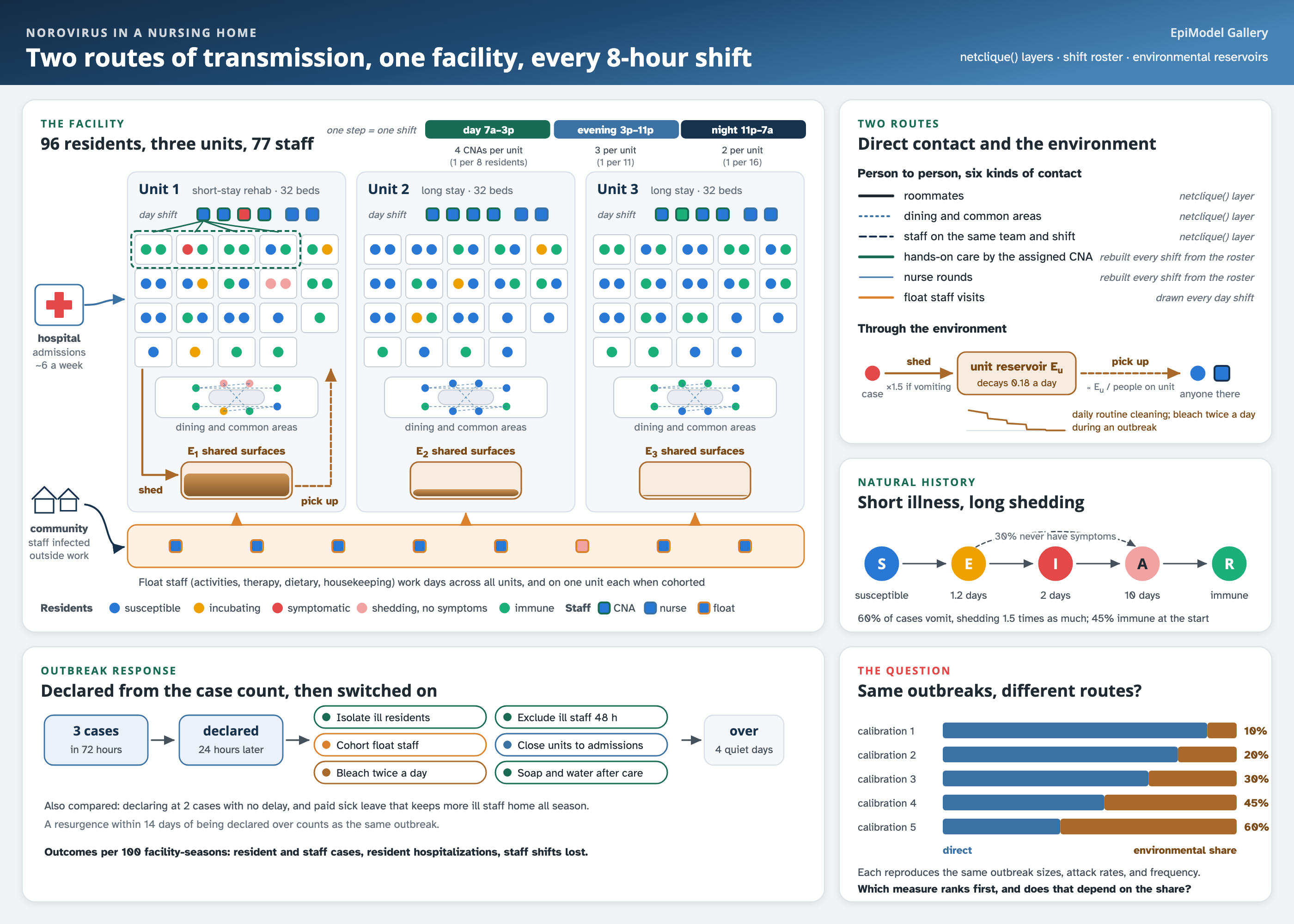
An enteric example: norovirus in a 96-bed nursing home in 8-hour shifts, spreading through shared rooms, dining areas, staff teams, and hands-on care, and through each unit’s contaminated surfaces. Rooms, units, and staff teams are netclique() layers; care contacts are rebuilt every shift from a weekly roster; each unit carries an environmental reservoir; and outbreak control switches on when the facility’s own case count crosses a threshold. It compares isolation, exclusion, cohorting, closure, cleaning, and hand hygiene, then recalibrates the model at five environmental shares of transmission that reproduce the same outbreaks and asks whether the ranking of the measures holds.
Overview
Norovirus causes most outbreaks of acute gastroenteritis in US long-term care facilities. Of the norovirus outbreaks reported in the United States in 2009 to 2018, 61% were in long-term care facilities; in a median outbreak, 29% of exposed residents and 11% of exposed staff became ill, and about 2 in every 100 cases were hospitalized (Calderwood et al. 2022). Reported outbreaks in these facilities had a median of 21 cases over 8 days in 2015 to 2025 (Calderwood and Mirza 2026).
Infected people shed very large amounts of virus in stool and vomit, and the virus stays infectious on hard surfaces for days. Norovirus therefore spreads both from person to person, through care, shared rooms, and shared tables, and through the environment, from rails, tables, and bathrooms that an infected person has contaminated. How transmission divides between the two routes has not been measured (Lopman et al. 2012). Population-level norovirus models assume direct transmission (Gaythorpe et al. 2018), and the one model that separated the routes, fitted to an outbreak on a cruise ship, attributed roughly 10 to 30% of the reproduction number to the environment (Towers et al. 2018). The split matters for control. Isolating ill residents and excluding ill staff remove infectious people from contact; cleaning removes virus from surfaces. The empirical record cannot rank these measures: across 72 published outbreaks in semi-enclosed settings there was no detectable effect of control measures on outbreak duration or attack rate (Harris et al. 2010), because measures are applied together and more intensively in larger outbreaks.
This example builds a nursing home model in EpiModel with three features that no other Gallery example combines:
A facility built from clique layers and a shift roster. Each time step is one 8-hour shift. Residents live in double and single rooms on three units, one of them a short-stay rehabilitation unit, and staff work on a weekly roster. Roommates, residents of the same unit, and staff on the same team are three layers built with
netclique(), with no network model to fit. Care contacts between each resident and the nursing assistant and nurse assigned to them are built inside the infection module every shift from the roster, so that days off, relief staff, illness, and exclusion change who cares for whom. Residents are discharged and admitted into free beds throughout the season.An environmental reservoir on each unit. Each unit carries a level of contamination that infectious people add to, that decays, and that cleaning reduces in scheduled pulses, and everyone on the unit picks up infection from it. The reservoir is state that belongs to a place, not to a person, and is carried between time steps in
dat$run. This person-place layer is the core of an enteric model and the part of this example most worth reusing.Outbreak control that responds to the facility’s own case count. The facility declares an outbreak when cases cluster and declares it over when they stop, and control measures apply only while an outbreak is declared, as they do in practice.
The page has three parts. Part 1 runs a winter season with no control measures and checks it against US and European outbreak data. Part 2 compares six control measures, the main five together, the same bundle declared earlier, and paid sick leave. Part 3 recalibrates the model at five environmental shares of transmission, from 10% to 60%, each of which reproduces the same outbreaks, and compares the measures across them.
The question is the one an infection preventionist faces when cases appear on a unit: which measures prevent the most cases, and does the answer depend on a quantity that outbreak data cannot reveal?
NoteEpiModel features used here
- Three
netclique()layers (rooms, units, and staff teams) passed tonetsim()with nonetest()fit, andarrivals = "join"with anarrivals.FUNthat places each admitted resident in the room and unit of their bed. - Time steps of one shift, with contacts that depend on who is at work built inside a custom infection module from a weekly roster rather than stored as a network.
- State that belongs to places rather than people (each unit’s environmental reservoir, the current outbreak) carried between time steps in
dat$run, and outbreak records returned withsave.other. - An open population: discharges with
activeandexitTime, admissions withappend_core_attr()andappend_attr(). - Person-to-person transmissions recorded with
set_transmat()and extra columns; environmental infections counted withset_epi()because they have no infector. - Every season a single-simulation
netsim()call run in parallel withfuture.apply, so that scenarios share their random number streams season by season, and rare introductions sampled conditionally with a known weight.
NoteHow this relates to other norovirus models
The closest models of norovirus in long-term care are a stochastic compartmental model of a 100-bed French nursing home parameterized from observed contacts, which found that isolating symptomatic residents and raising staff hand hygiene each cut cases sharply but did not include the environment (Assab and Temime 2016), and analyses of US nursing home outbreak line lists that estimate who infected how many (Adams et al. 2020; Chen et al. 2023). Environmental transmission has been modeled in the environmental infection transmission system framework (Li et al. 2009), in a fomite model compared across venues including long-term care (Kraay et al. 2018), in the cruise ship model above, and in a network model of norovirus across schools, hospitals, care homes, and households in an English county (Rushton et al. 2019). We are not aware of a network model of norovirus inside a facility with an environmental reservoir on each unit. The parameters here are illustrative, the two transmission parameters are set to reproduce published outbreak sizes and frequency rather than fitted to any facility’s data, and the model is a template for building an enteric facility model, not a forecast.
TipDownload and run the standalone scripts
- model.R: main simulation script
- module-fx.R: custom module functions
model.R sources module-fx.R from examples/norovirus-nursing-home/ when run from the repository root. Sourcing the script interactively uses the full settings on this page (1,200 seasons for each of 36 scenarios), which take under an hour on ten cores. Rscript is not interactive and uses small continuous-integration settings whose results are not meant to be interpreted; to get the full settings from the command line, pass R code that defines run_full as the first argument:
Rscript model.R "run_full <- TRUE"Model Structure
Disease states
| Status | Description | Infectious? | Duration |
|---|---|---|---|
s |
Susceptible | No | |
e |
Infected, incubating | No | log-normal, median 1.2 days |
i |
Symptomatic; 60% vomit | Yes (1.5 times as much if vomiting) | gamma, mean 2 days |
a |
Shedding without symptoms, after symptoms end or in the 30% who never have them | 5% as much as i for residents, 1% for staff |
gamma, mean 10 days |
r |
Immune for the rest of the season | No |
The incubation period follows a meta-analysis (Lee et al. 2013), and illness lasts a median of about 2 days in nursing home residents and staff (Lopman et al. 2004). People without symptoms shed as much virus for as long as people with symptoms (Teunis et al. 2015) but transmit far less; following the community model of Simmons et al. (2013), shedding without symptoms is 5% as infectious per day for residents, which over 10 days adds about a quarter of a symptomatic case’s infectiousness. For staff it is 1%: in hospital outbreaks sampled in full, staff who shed without symptoms rarely transmitted, despite shedding as much virus (Sukhrie et al. 2012), which points to hygiene rather than biology. Cases who vomit infected 1.3 to 2.1 times as many others in US nursing home outbreaks (Adams et al. 2020; Chen et al. 2023), and vomiting is common (Kirby et al. 2016). At the start of the season, and on admission, 45% of people are immune: about 20% are genetically resistant to the common strains because they do not secrete the antigens the virus binds to (Thorvén et al. 2005), and immunity after infection lasts about five years (Simmons et al. 2013).
The facility
| Component | Model | Basis |
|---|---|---|
| Residents | 96 in 3 units of 32 beds: 13 double rooms and 6 single rooms per unit | median US facility has 100 certified beds; about 80% of Medicare stays are in semi-private rooms (CMS provider data; Zhu et al. 2022) |
| Turnover | mean stay 40 days on unit 1 (short-stay rehabilitation), 2 years on units 2 and 3; free beds refilled at 50% a day; about 6 admissions a week | 0.88 admissions per 100 resident-days (CMS cost reports, 2023) |
| Nursing assistants (CNAs) | care groups of 8 beds on days, about 11 on evenings, 16 on nights: 4, 3, and 2 CNAs per unit; 42 on the roster | 2.25 CNA hours per resident day, the US median (CMS Payroll-Based Journal, 2026) |
| Licensed nurses | 2, 1, and 1 per unit by shift; each sees part of the unit every shift; 21 on the roster | |
| Float staff | 14 (activities, therapy, dietary, housekeeping) on days, across all units | in one Spanish nursing home, 45% of staff were not assigned to a floor (Parrón et al. 2019) |
| Roster | each staff member has two fixed days off a week; relief staff in each pool cover care groups whose usual CNA is off or ill, and when no relief is left another CNA on the unit takes on the group |
Contacts
Contact is weighted by hours of close contact per pair per shift, with hands-on care counted at a higher weight because it involves contact with stool and vomit. The weights are illustrative, informed by proximity-sensor studies in long-term care, in which residents spent most of their contact time with other residents and resident-to-resident contact peaked at meal times (Duval et al. 2018; Champredon et al. 2018).
| Contact | Who | Weight per pair (day, evening, night) | How it is built |
|---|---|---|---|
| Roommates | residents sharing a room | 1, 1, 1 | netclique() layer on room |
| Dining and common areas | residents of the same unit, unless isolated | 0.03, 0.02, 0 | netclique() layer on res_unit |
| Staff team | staff of the same unit and shift, or the float team, both at work | 0.1, 0.1, 0.1 | netclique() layer on team |
| Care | each resident and the CNA covering their care group | 0.5, 0.35, 0.2 | built each shift from the roster |
| Nurse rounds | each resident and the nurse covering their part of the unit | 0.1, 0.05, 0.03 | built each shift from the roster |
| Float staff | each float staff member and 6 residents a shift | 0.2 on days | drawn each day shift |
The environment
Each unit \(u\) has a reservoir \(E_u\) in arbitrary units. In each shift, every infectious person on the unit adds to it in proportion to their infectiousness (1 for a symptomatic case, 1.5 if vomiting, 0.05 for residents and 0.01 for staff without symptoms) and their time on the unit; float staff divide their shift among the units. The reservoir decays at 0.18 a day, a half-life of about four days, the rate measured for the infectivity of murine norovirus on stainless steel over several weeks (Kim et al. 2014; Fallahi and Mattison 2011). Routine cleaning at the start of each day shift removes 30% of it, reflecting the finding that detergent wiping leaves much of the virus in place (Barker et al. 2004), and hypochlorite cleaning during an outbreak removes 60% at the start of the day and evening shifts. Hypochlorite inactivates norovirus surrogates on clean test surfaces, but not every contaminated surface is reached, and on soiled surfaces without precleaning virus remained on up to 28% of them (Barker et al. 2004); 60% per cleaning is a judgment between the two. A susceptible person on the unit is infected from it at hazard
\[ \lambda_{\text{env}} = w \, \frac{E_u}{N_u}, \]
where \(w\) is the person’s time on the unit’s shared surfaces in the shift and \(N_u\) the number of people on the unit. Dividing by \(N_u\) makes the route frequency dependent, as for small, frequently touched surfaces (Li et al. 2009). Hands are folded into the reservoir rather than tracked separately: the share of shed virus that reaches hands, and the rates at which hands and surfaces exchange it, have no norovirus data behind them (Kraay et al. 2018).
Person-to-person and environmental exposures compete within each shift. Each exposure \(k\) of a susceptible person carries a hazard \(\lambda_k\) (for a contact, \(\beta \, w_k\) times the infector’s infectiousness and any precaution multiplier), draws an exponential waiting time, and the first arrival inside the shift, if any, infects the person and is recorded as the route. The probability of infection is \(1 - \exp(-\sum_k \lambda_k)\) and each route’s share is proportional to its hazard. Because deposition and pickup enter only as a product, the scale of \(E_u\) is arbitrary; one parameter, env.dep, sets the strength of the environmental route, and beta sets the strength of direct transmission.
Introductions
Norovirus enters in two ways: staff infected in the community, and infected residents admitted from hospitals or the community, at rates that rise and fall with a winter season peaking in mid-January (75% of US long-term care outbreaks begin in December to March; Calderwood et al. 2022). An infected admission was infected at a random time before arrival, so most arrive shedding without symptoms after their illness, some arrive incubating, and a few arrive with symptoms; those are placed on contact precautions in their room on arrival, as transfer protocols require. No study has measured how often each route seeds an outbreak, so the split of introductions, about two thirds through staff, is an assumption. The overall rate is set so that the model produces about 13 outbreaks per 100 facility-seasons, the rate Oregon found when it investigated outbreaks in every long-term care facility (Rosenthal et al. 2011); the national reported rate, 4.1 per 100 facilities a year, is a lower bound, and England’s, corrected for underreporting, is 32 gastroenteritis outbreaks per 100 care homes a year (Inns et al. 2019). Part 1 returns to what this rate implies.
At that rate most seasons have no introduction at all, and a season without one has no cases under any policy. Simulating those seasons would spend most of the run time producing zeros, so each simulated season draws its introductions before it runs, conditional on at least one, and every season-level result is weighted by the probability of at least one, \(1 - e^{-\Lambda}\), where \(\Lambda\) is the expected number of introductions in a season. The estimate is unbiased, and its Monte Carlo error is several times smaller for the same run time.
Outbreak declaration and control measures
The facility declares an outbreak 24 hours after 3 or more residents or staff have had symptom onset within 72 hours, the threshold in Wisconsin’s guidance for long-term care facilities (Department of Health Services publication P-00653, 2017); state rules range from 2 cases in 48 hours to 3 residents in 7 days. It declares the outbreak over after 4 days without a new onset, Maryland’s rule. A resurgence declared within 14 days of the end counts as the same outbreak. While an outbreak is declared, the measures switched on apply. Each follows the 2011 guideline of the Healthcare Infection Control Practices Advisory Committee (MacCannell et al. 2011):
| Measure | In the model |
|---|---|
| Isolate ill residents | every resident who becomes ill stays in their room (no dining or common-area contact) and receives care with contact precautions that halve care transmission, until 48 hours after symptoms end; without this, only residents who arrive ill are isolated |
| Exclude ill staff | symptomatic staff stay home until 48 hours after symptoms end; without this, 30% of symptomatic staff keep working, as 28.5% of long-term care staff with influenza-like illness did (Chiu et al. 2017) |
| Cohort float staff | each float staff member works on one unit only |
| Close units to admissions | no admissions to units with a case in the outbreak |
| Bleach twice a day | hypochlorite cleaning at the start of the day and evening shifts on every unit |
| Soap and water after care | staff hands carry 20% less: care, nurse, and float-staff contact transmits 20% less, and staff shed 20% less onto surfaces and pick up 20% less from them |
Paid sick leave, the one policy that acts before any outbreak is declared, lowers the share of symptomatic staff who work from 30% to 10% all season; paid sick leave was associated with a 62% lower risk of outbreaks in New York nursing homes (Li et al. 1996). Earlier declaration applies the five main measures after 2 cases in 48 hours, with no reporting delay.
Setup
# The custom modules used in control.net() and their excerpts below.
source("module-fx.R")
Building the Facility
Residents, rooms, and the staff roster
# Three units of 32 beds: 13 double rooms (beds 1 to 26) and 6 single rooms
# (beds 27 to 32). Unit 1 is the short-stay rehabilitation unit.
n.units <- 3
beds.per.unit <- 32
res_unit <- rep(seq_len(n.units), each = beds.per.unit)
res_bed <- rep(seq_len(beds.per.unit), n.units)
room_in_unit <- ifelse(res_bed <= 26, (res_bed + 1) %/% 2, 13 + (res_bed - 26))
res_room <- (res_unit - 1) * 19 + room_in_unit

# Staff pools. Each unit has a pool of nursing assistants (CNAs) and of
# licensed nurses for each shift, sized so that the pool covers the shift's
# care groups every day of the week when each member takes two days off.
# Float staff (activities, therapy, dietary, housekeeping) work days across
# all units.
cna_pool <- c(day = 6, evening = 5, night = 3)
nurse_pool <- c(day = 3, evening = 2, night = 2)
n_float <- 14
staff <- do.call(rbind, lapply(seq_len(n.units), function(u) {
  do.call(rbind, lapply(1:3, function(sh) {
    rbind(data.frame(role = "cna", unit = u, staff_shift = sh,
                     pool_k = seq_len(cna_pool[sh])),
          data.frame(role = "nurse", unit = u, staff_shift = sh,
                     pool_k = seq_len(nurse_pool[sh])))
  }))
}))
staff <- rbind(staff, data.frame(role = "float", unit = 0, staff_shift = 1,
                                 pool_k = seq_len(n_float)))
# Two days off a week, staggered across each pool.
staff$off1 <- ((2 * staff$pool_k - 2) %% 7) + 1
staff$off2 <- ((2 * staff$pool_k - 1) %% 7) + 1
staff$team <- ifelse(staff$role == "float", "float",
                     paste0("u", staff$unit, "s", staff$staff_shift))
staff$float_unit <- ifelse(staff$role == "float",
                           (staff$pool_k - 1) %% n.units + 1, NA)

n_res <- length(res_unit)
n_staff <- nrow(staff)
n <- n_res + n_staff
table(staff$role, staff$staff_shift)
         1  2  3
  cna   18 15  9
  float 14  0  0
  nurse  9  6  6
The roster gives each unit 4 CNAs and 2 nurses on the day shift on most days, and the pools are sized so that a care group is covered even when its usual CNA is off: six day-shift CNAs with two days off each leave four or five at work every day.
Three clique layers
# Every attribute any module reads is set on the base network, so netsim()
# copies it into the simulation. Residents have no staff attributes and staff
# no room or bed.
nw <- network_initialize(n)
attrs <- list(
  type = c(rep("res", n_res), rep("staff", n_staff)),
  role = c(rep("resident", n_res), staff$role),
  unit = c(res_unit, staff$unit),
  res_unit = c(res_unit, rep(NA, n_staff)),
  room = c(res_room, rep(NA, n_staff)),
  bed = c(res_bed, rep(NA, n_staff)),
  team = c(rep(NA, n_res), staff$team),
  staff_id = c(rep(NA, n_res), seq_len(n_staff)),
  staff_shift = c(rep(NA, n_res), staff$staff_shift),
  pool_k = c(rep(NA, n_res), staff$pool_k),
  off1 = c(rep(NA, n_res), staff$off1),
  off2 = c(rep(NA, n_res), staff$off2),
  float_unit = c(rep(NA, n_res), staff$float_unit),
  infRoute = rep(NA_character_, n),
  stage_end = rep(NA_real_, n),
  carer = rep(NA_real_, n),
  nurse_of = rep(NA_real_, n),
  onsetTime = rep(NA_real_, n),
  symEnd = rep(NA_real_, n),
  hold_until = rep(NA_real_, n),
  on_duty = rep(0, n),
  vomit = rep(0, n),
  presentee = rep(0, n),
  isolated = rep(0, n),
  excluded = rep(0, n)
)
for (a in names(attrs)) nw <- set_vertex_attribute(nw, a, attrs[[a]])

# Three clique layers: roommates, residents of the same unit, and staff on
# the same team. A new resident joins the room and unit of the bed they are
# admitted to, which the admission module writes to their attributes.
room_back <- function(dat, at, new_ids, network) get_attr(dat, "room")[new_ids]
unit_back <- function(dat, at, new_ids, network) get_attr(dat, "res_unit")[new_ids]
est_room <- netclique(nw, group.attr = "room", arrivals = "join",
                      arrivals.FUN = room_back)
est_unit <- netclique(nw, group.attr = "res_unit", arrivals = "join",
                      arrivals.FUN = unit_back)
est_team <- netclique(nw, group.attr = "team")
layers <- list(est_room, est_unit, est_team)
A clique layer has no formation model and is never resimulated: every pair of nodes that share a value of the grouping attribute is an edge, and nodes with NA are isolates. Residents carry a room and a unit and no team; staff carry a team and no room. When a resident is discharged, the node leaves with its edges; when a new resident is admitted, the admission module writes the room and unit of the free bed into the new node’s attributes, and each layer’s arrivals.FUN reads them back so that the node joins the right room and unit.
Custom Modules
Seven custom modules run in each shift: staffing (who is at work, and who cares for whom), infect (every route of transmission), environ (the reservoirs), progress (natural history), outbreak (declaration and control), discharge, and admit. Full code is in module-fx.R; the parts that carry the model’s logic are below.
staffing: the shift clock and the care assignment
1shift <- (at - 1) %% 3 + 1
weekday <- ((at - 1) %/% 3) %% 7 + 1
2absent <- (status == "i" & presentee == 0) | excluded == 1
scheduled <- is_staff & staff_shift == shift &
  weekday != off1 & weekday != off2
on_duty <- as.numeric(scheduled & !absent)

3prim <- match(seq_len(groups), pool_k[cnas])
cover[!is.na(prim)] <- staff_id[cnas[prim[!is.na(prim)]]]
relief <- cnas[pool_k[cnas] > groups]
gaps <- which(is.na(cover))
n_fill <- min(length(gaps), length(relief))
if (n_fill > 0) cover[gaps[seq_len(n_fill)]] <- staff_id[relief[seq_len(n_fill)]]
gaps <- which(is.na(cover))
if (length(gaps) > 0) {
  cover[gaps] <- staff_id[cnas[(seq_along(gaps) - 1) %% length(cnas) + 1]]
}
4grp <- ceiling(bed[res_u] / (beds.per.unit / groups))
carer[res_u] <- cover[grp]- 1
-
The clock. Step
atis one of three shifts on one day of the week; nothing else in the model needs to know the time of day. - 2
- Who is at work. A staff member works their shift unless it is a day off, they are symptomatic and staying home, or they are excluded.
- 3
- Coverage. Pool member k is the usual CNA for care group k; relief members fill the groups of anyone absent; groups still uncovered are added to the load of a CNA already on the unit.
- 4
- By bed, by id. Care groups belong to beds, so a new resident inherits their bed’s group, and assignments are stored as staff ids rather than node positions, which shift when residents are discharged.
infect: every route in one module
1add_pairs <- function(rows, a, b, w, route) {
  w <- rep_len(w, length(a))
  inf <- c(a, b)
  rec <- c(b, a)
  ww <- c(w, w)
  keep <- infness[inf] > 0 & sus[rec] & ww > 0
  rows[[length(rows) + 1]] <- list(
    sus = rec[keep], inf = inf[keep], route = rep(route, sum(keep)),
    lambda = beta * ww[keep] * infness[inf[keep]])
  return(rows)
}
2el <- get_edgelist(dat, network = 1)
rows <- add_pairs(rows, el[, 1], el[, 2], w.room, "room")
3res_ids <- which(is_res & !is.na(carer))
cna_pos <- match(carer[res_ids], staff_id)
mult <- ifelse(isolated[res_ids] == 1, prec.mult, 1) * hands
rows <- add_pairs(rows, res_ids, cna_pos, w.care * mult, "care")
4rows[[length(rows) + 1]] <- list(
  sus = j, inf = rep(NA_integer_, length(j)), route = rep("env", length(j)),
  lambda = w_on[j, u] * env[u] / n_on[u])
5t <- rexp(length(pos), rate = lambda[pos])
hit <- pos[t < 1]
ex <- ex[order(ex$sus, ex$t), , drop = FALSE]
ex <- ex[!duplicated(ex$sus), , drop = FALSE]- 1
-
One hazard per exposure. Each pair is checked in both directions, and an infectious-to-susceptible exposure carries a hazard of
betatimes its contact weight times the infector’s infectiousness. - 2
-
Clique layers. The roommate, unit, and team layers are read with
get_edgelist()like any other layer; the unit layer drops isolated residents and the team layer keeps pairs where both are at work. - 3
-
Care from the roster. Care contacts are the pairs of each resident and the staff member in their
carerattribute, with contact precautions for isolated residents and the hand hygiene multiplier during an outbreak with soap and water. - 4
- The reservoir. Every susceptible person on a contaminated unit has one environmental exposure, with no infector.
- 5
-
Competing exposures. Each exposure draws an exponential waiting time with its hazard; a person is infected if the first arrival falls inside the shift, and that exposure is the route. Person-to-person infections go to
set_transmat(); environmental ones are counted by route.
environ: deposition, decay, and cleaning
for (u in seq_len(n.units)) {
1  dep <- sum(shed[is_res & unit == u]) * env.w.res +
    sum(shed[present & type == "staff" & role != "float" & unit == u])
  if (cohort) {
    dep <- dep + sum(shed[present & role == "float" & float_unit == u])
  } else {
    dep <- dep + sum(shed[present & role == "float"]) / n.units
  }
2  env[u] <- env[u] * exp(-env.decay / 3) + env.dep * dep
}
3if (shift == 1) env <- env * (1 - clean.routine)
if (bleach && shift %in% c(1, 2)) env <- env * (1 - clean.bleach)
4dat$run$env <- env- 1
- Deposition. Infectious residents shed on their own unit, unit staff on theirs, and float staff a third of their shift on each unit, or all of it on one unit while cohorted.
- 2
- Decay. A third of the daily rate per shift.
- 3
- Cleaning as pulses. Routine cleaning at the start of each day shift, and hypochlorite at the start of the day and evening shifts during an outbreak with enhanced cleaning. Cleaning at known times, rather than as a faster decay rate, gives the environmental route a timing of its own, which Part 3 returns to.
- 4
-
Place state. The reservoir is not a node attribute; it is a vector carried from step to step in
dat$run, where netsim keeps anything a module needs between steps.
outbreak: declaration, resurgence, and the end of an outbreak
if (is.null(ob) || !ob$active) {
1  if (is.null(dat$run$pending) && sum(on_at > at - trig.window) >= trig.n) {
    dat$run$pending <- at + trig.delay
  }
  if (!is.null(dat$run$pending) && at >= dat$run$pending) {
    dat$run$pending <- NULL
2    if (is.null(ob)) {
      ob <- list(first = min(on_at[on_at > at - trig.window - trig.delay]),
                 declared = at, declarations = 0)
    }
    ob$active <- TRUE
    ob$declarations <- ob$declarations + 1
  }
3} else if (sum(on_at > at - end.window) == 0) {
  ob$active <- FALSE
  ob$over <- at
}- 1
-
The trigger. Onsets are read from a log kept by
progressindat$run$onsets, which keeps residents who have since been discharged. - 2
- New or resurging. An outbreak that is over but has not yet stayed over for 14 days is still the current outbreak, so a resurgence reopens it.
- 3
- The end. No onset in 4 days ends the outbreak and lifts the measures; people already isolated or excluded stay so until 48 hours after their symptoms end.
Module order
module.order = c("resim_nets.FUN", "summary_nets.FUN", "staffing.FUN",
                 "infection.FUN", "environ.FUN", "progress.FUN",
                 "outbreak.FUN", "departures.FUN", "arrivals.FUN",
                 "nwupdate.FUN")
Staffing runs first, so that transmission in a shift involves the staff at work in it. Infection reads the reservoirs as they stood at the end of the previous shift, and environ then adds this shift’s shedding and applies decay and cleaning. Discharges and admissions run on day shifts only, before nwupdate.FUN updates the clique layers. With only clique layers, resim_nets.FUN and summary_nets.FUN do nothing, but leaving them out of the order raises a warning.
Parameters
Natural history and severity. The disease parameters are in the table under Disease states. Severity is applied to resident cases after the simulation: 3.4% are hospitalized and 0.37% die, the US long-term care rates of 21.6 hospitalizations and 2.3 deaths per 1,000 cases (Calderwood et al. 2022) assigned to residents, who are 63% of cases (Chen et al. 2023).
What was set to reproduce outbreak data. Three parameters were chosen by simulation rather than taken from the literature: beta, the strength of person-to-person transmission per contact-hour; env.dep, the strength of the environmental route; and intro.staff, the rate of introductions (with intro.adm held at the ratio that makes about a third of introductions arrive with admissions). They were chosen in two steps. Runs of single introductions into an otherwise quiet facility fixed the ratio of beta to env.dep for each target environmental share and scaled both until the median outbreak, with no control measures, had about 21 to 23 cases. Season runs then set the introduction rate to give about 13 outbreaks per 100 facility-seasons. The five resulting pairs of beta and env.dep are in calib, and Part 3 checks that each reproduces the same outbreaks; Parts 1 and 2 use the middle one, in which about 30% of transmission is environmental. The environmental decay rate, the cleaning fractions, the contact weights, and the roster were set from the literature or by judgment and not adjusted.
| Parameter | Value | Meaning | Basis |
|---|---|---|---|
inc.meanlog, inc.sdlog |
0.182, 0.495 | log-normal incubation, median 1.2 days | Lee et al. 2013 |
sym.mean |
2 days | symptomatic period (gamma, shape 4) | Lopman et al. 2004 |
shed.mean |
10 days | shedding without symptoms (gamma, shape 2) | Simmons et al. 2013 |
p.asym |
0.3 | infections that never have symptoms | CDC 2011; challenge studies |
rel.inf.a |
0.05, 0.01 | infectiousness without symptoms, relative to symptoms: residents, staff | Simmons et al. 2013; Sukhrie et al. 2012 |
p.vomit, vomit.mult |
0.6, 1.5 | cases who vomit, and their relative infectiousness and shedding | Kirby et al. 2016; Adams et al. 2020; Chen et al. 2023 |
p.immune |
0.45 | immune at the start of the season and on admission | Thorvén et al. 2005; Simmons et al. 2013 |
beta |
0.67 | person-to-person transmission per weighted contact-hour | set to reproduce outbreak size |
env.dep |
0.149 | strength of the environmental route | set to reproduce outbreak size at a 30% share |
env.decay |
0.18 per day | decay of the reservoir | Kim et al. 2014; Fallahi and Mattison 2011 |
clean.routine, clean.bleach |
0.3, 0.6 | share of the reservoir removed by routine cleaning (daily) and hypochlorite (twice daily in outbreaks) | Barker et al. 2004; judgment |
p.present |
0.3 | symptomatic staff who keep working without exclusion | Chiu et al. 2017 |
prec.mult, hh.mult |
0.5, 0.8 | care transmission with contact precautions; transmission through staff hands with soap and water | judgment |
intro.staff, intro.adm |
7.9e-5, 1.86e-3 | exposures outside the facility per staff member per day, and infected admissions per admission, at the peak of the season | set to about 13 outbreaks per 100 facility-seasons (Rosenthal et al. 2011) |
los |
40, 730, 730 days | mean length of stay by unit | CMS cost reports |
trig.n, trig.window, trig.delay |
3 onsets, 72 hours, 24 hours | outbreak declaration | Wisconsin guidance; Davis et al. 2011 |
ImportantSimplifications
- One reservoir per unit, and no hands. A unit’s rooms, bathrooms, dining room, and equipment share one level of contamination, so a vomiting episode in one room raises the risk in every room equally. Hands are folded into the reservoir: staff who are not infected do not carry virus from one resident to the next on their hands, which caps what hand hygiene can do in this model.
- No individual precautions before an outbreak. Residents who arrive ill are isolated, but residents who become ill in the facility are isolated only once an outbreak is declared.
- First-order decay. Norovirus surrogates decay quickly at first and then slowly on dry surfaces; a single rate overstates early loss and understates the long tail.
- No visitors, food, or water. Visitors are not modeled, and food- and water-borne introductions, under 1% of US long-term care outbreaks, are left out.
- One genotype, one season. Immunity is fixed for the season, and the immune share does not respond to a strain new to the population, such as GII.17 in 2024 to 2025.
- Staff live nowhere. Staff are infected in the community at a set rate, and infection does not pass from the facility to their households and back.
- No calibration to a facility. The transmission parameters reproduce the size and frequency of published outbreaks; they are not fitted to any facility’s line list.
# Vectors of three are values for the day, evening, and night shifts, and
# rel.inf.a holds values for residents and staff. Contact weights are hours of
# close contact per pair per shift, with hands-on care weighted up for contact
# with stool and vomit. beta and env.dep, the two
# transmission parameters, are set in Part 3 by the calibration chosen there.
param_base <- list(
  # facility and staffing
  n.units = n.units, beds.per.unit = beds.per.unit, cna.groups = c(4, 3, 2),
  los = c(40, 730, 730), fill.prob = 0.5,
  # natural history (days)
  inc.meanlog = 0.182, inc.sdlog = 0.495,
  sym.mean = 2, sym.shape = 4, shed.mean = 10, shed.shape = 2,
  p.asym = 0.3, p.vomit = 0.6, p.immune = 0.45,
  # person-to-person transmission
  beta = NA, rel.inf.a = c(0.05, 0.01), vomit.mult = 1.5,
  w.room = c(1, 1, 1), w.common = c(0.03, 0.02, 0), w.team = c(0.1, 0.1, 0.1),
  w.care = c(0.5, 0.35, 0.2), w.nurse = c(0.1, 0.05, 0.03),
  w.float = c(0.2, 0, 0), n.float.res = 6,
  # environment
  env.dep = NA, env.decay = 0.18, env.w.res = c(1, 1, 0.25),
  clean.routine = 0.3, clean.bleach = 0.6,
  # introductions (per staff member per day, and per admission, at the peak)
  intro.staff = 7.9e-5, intro.adm = 1.86e-3, season.peak = 76, season.sd = 45,
  # staff who work while ill
  p.present = 0.3,
  # outbreak declaration
  trig.n = 3, trig.window = 9, trig.delay = 3, end.window = 12, ob.gap = 42,
  # control measures (all off) and their settings
  ctl.isolate = 0, ctl.exclude = 0, ctl.cohort = 0, ctl.close = 0,
  ctl.clean = 0, ctl.handhyg = 0,
  iso.hold = 6, excl.hold = 6, prec.mult = 0.5, hh.mult = 0.8
)

# Five calibrations that reproduce the same outbreaks with different shares
# of transmission through the environment (Part 3). The page's main analysis
# uses the middle one.
calib <- data.frame(
  share = c(0.10, 0.20, 0.30, 0.45, 0.60),
  beta = c(0.935, 0.796, 0.670, 0.490, 0.317),
  env.dep = c(0.0520, 0.1010, 0.1485, 0.2205, 0.2894)
)
central <- 3
param_base$beta <- calib$beta[central]
param_base$env.dep <- calib$env.dep[central]
Running Seasons
# Norovirus enters through staff exposed in the community and through new
# admissions, at rates that follow a winter season peaking in mid-January.
# Introductions are rare: at these rates most seasons have none, and a season
# without one has no cases under any policy. Each simulated season therefore
# draws its introductions before it runs, conditional on at least one, and
# season-level results are weighted by the probability of at least one,
# 1 - exp(-Lambda), where Lambda is the expected number per season.
adm_per_day <- sum(beds.per.unit * (1 - exp(-1 / param_base$los)))
draw_intros <- function(p, ndays) {
  season <- exp(-(seq_len(ndays) - p$season.peak)^2 / (2 * p$season.sd^2))
  rate <- c(p$intro.staff * n_staff * season, p$intro.adm * adm_per_day * season)
  Lambda <- sum(rate)
  k <- qpois(runif(1, ppois(0, Lambda), 1), Lambda)
  ev <- sample.int(length(rate), k, replace = TRUE, prob = rate)
  list(staff = ev[ev <= ndays], adm = ev[ev > ndays] - ndays,
       weight = 1 - exp(-Lambda))
}
control <- control.net(
type = NULL, nsteps = nsteps, nsims = 1, ncores = 1,
tergmLite = TRUE, resimulate.network = TRUE, save.nwstats = FALSE,
staffing.FUN = staffing,
infection.FUN = infect,
environ.FUN = environ,
progress.FUN = progress,
outbreak.FUN = outbreak,
departures.FUN = discharge,
arrivals.FUN = admit,
module.order = c("resim_nets.FUN", "summary_nets.FUN", "staffing.FUN",
"infection.FUN", "environ.FUN", "progress.FUN",
"outbreak.FUN", "departures.FUN", "arrivals.FUN",
"nwupdate.FUN"),
save.other = "ob_log",
verbose = FALSE
)# Each season is its own single-simulation netsim() call, run in parallel. A
# fixed future.seed gives season s the same random number stream in every
# scenario, so scenarios share their introductions and differ only once
# their control measures first act. Each season returns its totals, its
# outbreaks, and the daily onsets of each outbreak from its first case (NA
# past the end of the season).
routes <- c("room", "common", "team", "care", "nurse", "float")
run_scenario <- function(changes = list(), nsims, keep_epi = 0, seed = 2026) {
p <- modifyList(param_base, changes)
one <- function(s) {
intro <- draw_intros(p, ndays)
param <- do.call(param.net, c(p, list(intro.staff.days = intro$staff,
intro.adm.days = intro$adm)))
status0 <- ifelse(runif(n) < p$p.immune, "r", "s")
sim <- netsim(layers, param, init.net(status.vector = status0), control)
d <- as.data.frame(sim)
d[is.na(d)] <- 0
res_on <- d$onset.res.u1 + d$onset.res.u2 + d$onset.res.u3
tot <- c(res_cases = sum(res_on), staff_cases = sum(d$onset.staff),
colSums(d[, paste0("inf.", routes)]),
inf.env.res = sum(d$inf.env.res), inf.env.staff = sum(d$inf.env.staff),
intro_staff = sum(d$intro.staff), intro_adm = sum(d$intro.adm),
staff_shifts_lost = sum(d$staff.absent),
ob_days = sum(d$ob.active) / 3, admissions = sum(d$admissions),
outbreaks = NROW(sim$ob_log[[1]]))
# Person-to-person transmissions by route and by who infected whom.
tm <- as.data.frame(get_transmat(sim))
pairs <- c("res>res", "staff>res", "res>staff", "staff>staff")
by_route <- paste0(rep(routes, each = 2), ".", c("res", "staff"))
who <- setNames(numeric(length(pairs) + length(by_route)), c(pairs, by_route))
if (nrow(tm) > 0) {
who[pairs] <- table(factor(paste(tm$infType, tm$susType, sep = ">"),
levels = pairs))
who[by_route] <- table(factor(paste(tm$route, tm$susType, sep = "."),
levels = by_route))
}
ob <- sim$ob_log[[1]]
curves <- NULL
if (NROW(ob) > 0) {
day_on <- tapply(res_on + d$onset.staff, (d$time - 1) %/% 3 + 1, sum)
curves <- t(sapply((ob$first - 1) %/% 3 + 1, function(d0) day_on[d0 + 0:39]))
ob$season <- s
}
list(tot = c(tot, who, weight = intro$weight), ob = ob, curves = curves,
epi = if (s <= keep_epi) d else NULL)
}
runs <- future.apply::future_lapply(seq_len(nsims), one, future.seed = seed)
list(tot = as.data.frame(do.call(rbind, lapply(runs, `[[`, "tot"))),
ob = do.call(rbind, lapply(runs, `[[`, "ob")),
curves = do.call(rbind, lapply(runs, `[[`, "curves")),
epi = lapply(runs, `[[`, "epi"))
}
if (ncores > 1) {
future::plan("multisession", workers = ncores)
} else {
future::plan("sequential")
}Analysis helpers
# A season total per 100 facility-seasons, with a 95% Monte Carlo interval.
per100 <- function(r, col) {
  x <- 100 * r$tot$weight * r$tot[[col]]
  m <- mean(x)
  h <- 1.96 * sd(x) / sqrt(length(x))
  c(mean = m, lo = m - h, hi = m + h)
}

# Percent change in a season total against a scenario run on the same random
# number streams, with a bootstrap interval that resamples seasons in pairs.
pct_change <- function(r, ref, col = "res_cases", B = 2000) {
  x <- r$tot[[col]]
  y <- ref$tot[[col]]
  est <- 100 * (sum(x) / sum(y) - 1)
  bs <- replicate(B, {
    i <- sample.int(length(x), replace = TRUE)
    100 * (sum(x[i]) / sum(y[i]) - 1)
  })
  c(est = est, lo = quantile(bs, 0.025, names = FALSE, na.rm = TRUE),
    hi = quantile(bs, 0.975, names = FALSE, na.rm = TRUE))
}

# One row per outbreak: size, attack rates among residents and staff of the
# units it touched (plus float staff), and duration from first to last onset.
staff_per_unit <- sum(staff$role != "float" & staff$unit == 1)
ob_stats <- function(r) {
  ob <- r$ob
  if (NROW(ob) == 0) {
    return(data.frame(size = numeric(0), ar_res = numeric(0), ar_staff = numeric(0),
                      days = numeric(0), units = numeric(0), resurged = logical(0)))
  }
  u <- pmax(ob$units, 1)
  data.frame(size = ob$cases.res + ob$cases.staff,
             ar_res = ob$cases.res / (beds.per.unit * u),
             ar_staff = ob$cases.staff / (staff_per_unit * u + n_float),
             days = (ob$last - ob$first) / 3,
             units = ob$units,
             resurged = ob$declarations > 1)
}

# Share of infections acquired in the facility that came from the environment.
env_share <- function(r) {
  env <- sum(r$tot$inf.env.res + r$tot$inf.env.staff)
  env / (env + sum(r$tot[, paste0("inf.", routes)]))
}

med_iqr <- function(x, digits = 0, pct = FALSE) {
  if (length(x) == 0) return("none")
  q <- quantile(x, c(0.5, 0.25, 0.75), names = FALSE) * if (pct) 100 else 1
  fmt <- paste0("%.", digits, "f [%.", digits, "f, %.", digits, "f]")
  sprintf(fmt, q[1], q[2], q[3])
}

# Severity among residents, per case (US long-term care outbreaks: 21.6
# hospitalizations and 2.3 deaths per 1,000 cases, 63% of cases residents).
p.hosp <- 0.034
p.death <- 0.0037
Part 1: A Season with No Control Measures
base <- run_scenario(nsims = nsims, keep_epi = min(nsims, 100))
ob_base <- ob_stats(base)
The baseline against outbreak data
The model produces 13.3 outbreaks per 100 facility-seasons from 0.53 introductions per season on average (an introduction here is a person infected outside the facility; exposures of people who are already immune do nothing). There are 25 outbreaks for every 100 introductions: in seasons with a single introduction, 20% of staff introductions and 35% of admission introductions led to a declared outbreak, and the rest ended with one or two cases or none. Most staff introductions end quietly because most ill staff stay home and staff shed without symptoms to little effect; most admission introductions end quietly because the admitted resident is past their illness.
The introduction rate that reproduces Oregon’s outbreak frequency implies that 0.8% of susceptible staff are infected outside work in a season. That is low: about 19 to 21 million people in the United States are ill with norovirus each year, about 6% of the population, most of them in winter (CDC). Either outbreaks are undercounted even under Oregon’s active surveillance, as they are in England, or real introductions start outbreaks less often than they do in this model. The model cannot tell which. The comparisons in Parts 2 and 3 are made outbreak by outbreak and depend little on the rate; the burden per facility-season scales with it.
The table compares the outbreaks with the targets. Outbreak size and the attack rate among residents of the affected units match US reports and Dutch ward-level data. The staff attack rate matches published outbreak reports but is about twice the median in US surveillance, which the surveillance authors note may undercount staff. Outbreaks last longer than the 8-day median in US surveillance, which counts many small outbreaks, and close to the 14.5-day median of published outbreaks in which no control measures were reported (Adams et al. 2022).
# The model against the targets.
targets <- data.frame(
  Quantity = c("Outbreaks per 100 facility-seasons",
               "Cases per outbreak, median [IQR]",
               "Resident attack rate on affected units (%)",
               "Staff attack rate (%)",
               "Residents as a share of cases (%)",
               "Duration, first to last onset (days)",
               "Units affected, mean"),
  Model = c(sprintf("%.1f", 100 * base$tot$weight[1] * mean(base$tot$outbreaks)),
            med_iqr(ob_base$size),
            med_iqr(ob_base$ar_res, pct = TRUE),
            med_iqr(ob_base$ar_staff, pct = TRUE),
            sprintf("%.0f", 100 * sum(base$tot$res_cases) /
                      sum(base$tot$res_cases + base$tot$staff_cases)),
            med_iqr(ob_base$days),
            sprintf("%.1f", mean(ob_base$units))),
  Reference = c("13 (Oregon, active surveillance); 4.1 (US reports, a lower bound)",
                "21 [11, 35] (US reports, 2015 to 2025)",
                "35.5 (Dutch wards, median)",
                "23.7 [11.6, 38.3] (published outbreaks); 10.9 (US reports)",
                "63 (107 US outbreaks)",
                "14.5 [9, 24.5] without measures (published); 8 to 13 (US reports)",
                "2.4 wards (Netherlands)")
)
knitr::kable(targets)| Quantity | Model | Reference |
|---|---|---|
| Outbreaks per 100 facility-seasons | 13.3 | 13 (Oregon, active surveillance); 4.1 (US reports, a lower bound) |
| Cases per outbreak, median [IQR] | 21 [17, 32] | 21 [11, 35] (US reports, 2015 to 2025) |
| Resident attack rate on affected units (%) | 38 [30, 47] | 35.5 (Dutch wards, median) |
| Staff attack rate (%) | 23 [14, 29] | 23.7 [11.6, 38.3] (published outbreaks); 10.9 (US reports) |
| Residents as a share of cases (%) | 59 | 63 (107 US outbreaks) |
| Duration, first to last onset (days) | 16 [12, 26] | 14.5 [9, 24.5] without measures (published); 8 to 13 (US reports) |
| Units affected, mean | 1.3 | 2.4 wards (Netherlands) |
# Burden per 100 facility-seasons.
burden <- rbind(
  "Resident cases" = per100(base, "res_cases"),
  "Resident hospitalizations" = p.hosp * per100(base, "res_cases"),
  "Resident deaths" = p.death * per100(base, "res_cases"),
  "Staff cases" = per100(base, "staff_cases"),
  "Staff shifts lost" = per100(base, "staff_shifts_lost")
)
knitr::kable(round(burden, 1), col.names = c("Mean", "Lower", "Upper"))| Mean | Lower | Upper | |
|---|---|---|---|
| Resident cases | 232.5 | 203.3 | 261.7 |
| Resident hospitalizations | 7.9 | 6.9 | 8.9 |
| Resident deaths | 0.9 | 0.8 | 1.0 |
| Staff cases | 158.7 | 141.7 | 175.8 |
| Staff shifts lost | 145.3 | 129.5 | 161.0 |
Per 100 facility-seasons, the model gives 233 resident cases (95% Monte Carlo interval 203 to 262), 7.9 resident hospitalizations, 0.9 resident deaths, 159 staff cases, and 145 staff shifts lost to illness.
Where infection happens
# Where infections happen: by route and by who was infected.
route_lab <- c(room = "Roommates", common = "Dining and common areas",
               team = "Staff team", care = "CNA care", nurse = "Nurse rounds",
               float = "Float staff", env = "Environment")
by_route <- rbind(
  Residents = c(colSums(base$tot[, paste0(routes, ".res")]), sum(base$tot$inf.env.res)),
  Staff = c(colSums(base$tot[, paste0(routes, ".staff")]), sum(base$tot$inf.env.staff))
)
colnames(by_route) <- route_lab
route_pct <- 100 * by_route / sum(by_route)
round(route_pct, 1)
Roommates Dining and common areas Staff team CNA care Nurse rounds
Residents 10 25.4 0.0 4.6 0.7
Staff 0 0.0 1.9 16.2 4.7
Float staff Environment
Residents 1.0 22.0
Staff 4.3 9.3who <- colSums(base$tot[, c("res>res", "staff>res", "res>staff", "staff>staff")])
round(100 * who / sum(who), 1) res>res staff>res res>staff staff>staff
51.6 9.1 36.6 2.7 Residents are most often infected by other residents: 52% of person-to-person transmissions are from resident to resident, 37% from residents to staff, and only 9% from staff to residents. Staff are the bridge into the facility, since two thirds of introductions arrive with them, but once norovirus is inside, residents carry it. This matches the direction of transmission reconstructed from a Dutch institutional outbreak, in which patients infected each other in 64% of recognized transmissions and staff had a reproduction number of 0.25 against 1.20 for patients (Heijne et al. 2012). The dining and common areas carry the most transmission among residents, and hands-on care carries most staff infections. In this calibration 31% of infections come from the environment, 35% of residents’ infections.
par(mfrow = c(1, 1), mar = c(4, 11, 1, 1))
ord <- order(colSums(route_pct))
barplot(route_pct[, ord], horiz = TRUE, las = 1, col = c("#2a78d6", "#d9822b"),
        border = NA, xlab = "Share of infections acquired in the facility (%)")
legend("bottomright", fill = c("#2a78d6", "#d9822b"), border = NA, bty = "n",
       legend = c("Residents infected", "Staff infected"))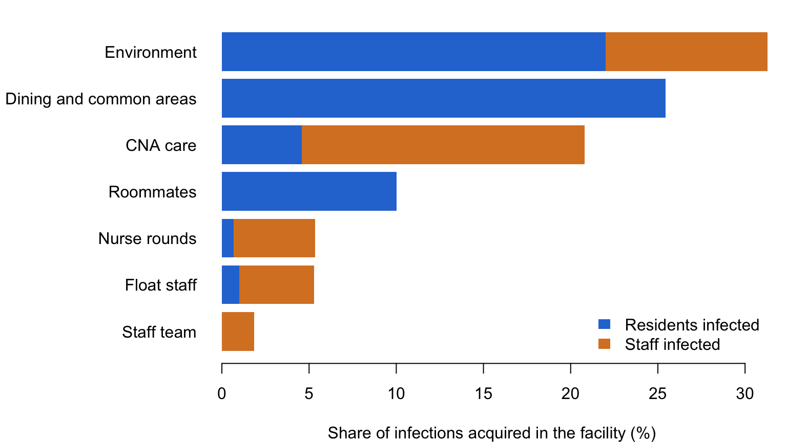
One outbreak, shift by shift
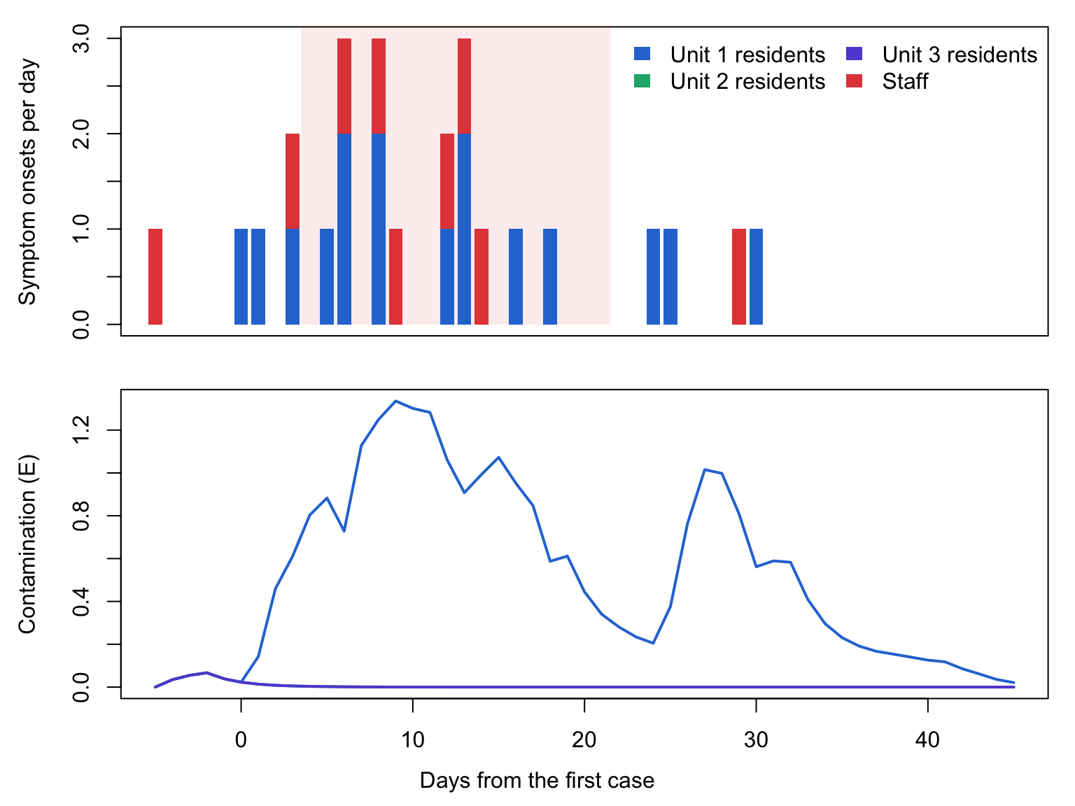
The figure follows one simulated season with an outbreak of about median size. The bars are symptom onsets each day by unit, the shaded band is the period in which the facility had declared an outbreak (with no measures in this scenario, declaration changes nothing), and the lower panel is each unit’s reservoir. Contamination rises with each symptomatic case, falls after routine cleaning each morning, and persists for days after the last case on a unit.
# One season with an outbreak of about median size and duration, day by day,
# from the seasons whose full output was kept.
kept <- which(!vapply(base$epi, is.null, logical(1)))
cand <- which(base$ob$season %in% kept)
if (length(cand) > 0) {
  dist <- abs(ob_base$size[cand] / median(ob_base$size) - 1) +
    abs(ob_base$days[cand] / median(ob_base$days) - 1)
  pick <- cand[which.min(dist)]
  ex <- base$epi[[base$ob$season[pick]]]
  ex$day <- (ex$time - 1) %/% 3 + 1
  daily <- aggregate(cbind(onset.res.u1, onset.res.u2, onset.res.u3, onset.staff,
                           ob.active) ~ day, data = ex, FUN = sum)
  env_day <- aggregate(cbind(env.u1, env.u2, env.u3) ~ day,
                       data = ex[ex$time %% 3 == 1, ], FUN = mean)
  first <- (base$ob$first[pick] - 1) %/% 3 + 1
  win <- daily$day >= first - 5 & daily$day <= first + 45
  x <- daily$day[win] - first
  bars <- as.matrix(daily[win, c("onset.res.u1", "onset.res.u2", "onset.res.u3",
                                 "onset.staff")])
  on <- daily$ob.active[win] > 0
  cols <- c("#2a78d6", "#1baf7a", "#6250d6", "#e34948")
  par(mfrow = c(2, 1), mar = c(1, 4.5, 1, 1), oma = c(3, 0, 0, 0))
  plot(NA, xlim = range(x), ylim = c(0, max(rowSums(bars), 1)), xaxt = "n",
       xlab = "", ylab = "Symptom onsets per day")
  if (any(on)) {
    rect(min(x[on]) - 0.5, 0, max(x[on]) + 0.5, par("usr")[4],
         col = adjustcolor("#e34948", 0.1), border = NA)
  }
  base_y <- rep(0, length(x))
  for (j in 1:4) {
    rect(x - 0.4, base_y, x + 0.4, base_y + bars[, j], col = cols[j], border = NA)
    base_y <- base_y + bars[, j]
  }
  legend("topright", fill = cols, border = NA, bty = "n", ncol = 2,
         legend = c("Unit 1 residents", "Unit 2 residents", "Unit 3 residents",
                    "Staff"))
  ew <- env_day$day >= first - 5 & env_day$day <= first + 45
  matplot(env_day$day[ew] - first, as.matrix(env_day[ew, -1]), type = "l", lty = 1,
          lwd = 2, col = cols[1:3], xlim = range(x), xlab = "",
          ylab = "Contamination (E)")
  mtext("Days from the first case", side = 1, line = 1.5, outer = TRUE)
}
Part 2: Control Measures
Each scenario switches on one measure, or a combination, while an outbreak is declared, and runs on the same seasons as the baseline: season s has the same introductions, at the same times, in every scenario, and the scenarios differ only from the moment their measures first act. Effects are therefore compared season by season, which removes most of the season-to-season noise from the comparison.
bundle <- list(ctl.isolate = 1, ctl.exclude = 1, ctl.cohort = 1, ctl.close = 1,
               ctl.clean = 1)
arms <- list(
  isolate = list(ctl.isolate = 1),
  exclude = list(ctl.exclude = 1),
  cohort = list(ctl.cohort = 1),
  close = list(ctl.close = 1),
  clean = list(ctl.clean = 1),
  handhyg = list(ctl.handhyg = 1),
  bundle = bundle,
  early = c(bundle, list(trig.n = 2, trig.window = 6, trig.delay = 0)),
  sickleave = list(p.present = 0.1)
)
arm_lab <- c(isolate = "Isolate ill residents", exclude = "Exclude ill staff",
             cohort = "Cohort float staff", close = "Close units to admissions",
             clean = "Bleach twice a day", handhyg = "Soap and water after care",
             bundle = "All five measures", early = "All five, declared earlier",
             sickleave = "Paid sick leave")
runs <- lapply(arms, function(a) run_scenario(a, nsims))
# The hand hygiene effect is an assumption; two more settings bracket it.
hh_runs <- list(
"0.95" = run_scenario(list(ctl.handhyg = 1, hh.mult = 0.95), nsims),
"0.8" = runs$handhyg,
"0.5" = run_scenario(list(ctl.handhyg = 1, hh.mult = 0.5), nsims)
)ctl_table <- do.call(rbind, lapply(names(arms), function(a) {
r <- runs[[a]]
pc <- pct_change(r, base)
ps <- pct_change(r, base, "staff_cases")
data.frame(
Scenario = arm_lab[[a]],
res = per100(r, "res_cases")[["mean"]],
res_pct = pc[["est"]], res_lo = pc[["lo"]], res_hi = pc[["hi"]],
staff_pct = ps[["est"]],
shifts = per100(r, "staff_shifts_lost")[["mean"]],
outbreaks = 100 * r$tot$weight[1] * mean(r$tot$outbreaks),
size = if (NROW(r$ob) > 0) median(ob_stats(r)$size) else NA
)
}))knitr::kable(
data.frame(Scenario = ctl_table$Scenario,
`Resident cases` = round(ctl_table$res),
`Change, residents (%)` = sprintf("%.0f [%.0f, %.0f]", ctl_table$res_pct,
ctl_table$res_lo, ctl_table$res_hi),
`Change, staff (%)` = round(ctl_table$staff_pct),
`Staff shifts lost` = round(ctl_table$shifts),
Outbreaks = round(ctl_table$outbreaks, 1),
`Cases per outbreak` = ctl_table$size, check.names = FALSE),
align = "lrrrrrr")| Scenario | Resident cases | Change, residents (%) | Change, staff (%) | Staff shifts lost | Outbreaks | Cases per outbreak |
|---|---|---|---|---|---|---|
| Isolate ill residents | 185 | -21 [-27, -15] | -22 | 112 | 13.3 | 18.0 |
| Exclude ill staff | 196 | -16 [-21, -10] | -14 | 284 | 14.0 | 19.0 |
| Cohort float staff | 201 | -14 [-20, -7] | -9 | 134 | 13.6 | 21.0 |
| Close units to admissions | 207 | -11 [-17, -4] | -4 | 140 | 13.8 | 19.5 |
| Bleach twice a day | 181 | -22 [-27, -16] | -20 | 118 | 14.3 | 17.0 |
| Soap and water after care | 216 | -7 [-13, -1] | -10 | 132 | 13.4 | 20.0 |
| All five measures | 131 | -43 [-48, -39] | -42 | 164 | 15.1 | 11.0 |
| All five, declared earlier | 93 | -60 [-64, -56] | -53 | 143 | 15.8 | 7.0 |
| Paid sick leave | 159 | -32 [-37, -26] | -27 | 138 | 10.5 | 20.0 |
par(mfrow = c(1, 1), mar = c(4, 13, 1, 1))
o <- order(ctl_table$res_pct, decreasing = TRUE)
y <- seq_along(o)
plot(ctl_table$res_pct[o], y, xlim = range(c(0, ctl_table$res_lo, ctl_table$res_hi),
                                         na.rm = TRUE), yaxt = "n", pch = 19,
     col = "#1a6b54", xlab = "Change in resident cases per season (%)", ylab = "")
segments(ctl_table$res_lo[o], y, ctl_table$res_hi[o], y, col = "#1a6b54", lwd = 2)
abline(v = 0, lty = 2, col = "gray50")
axis(2, at = y, labels = ctl_table$Scenario[o], las = 1, tick = FALSE)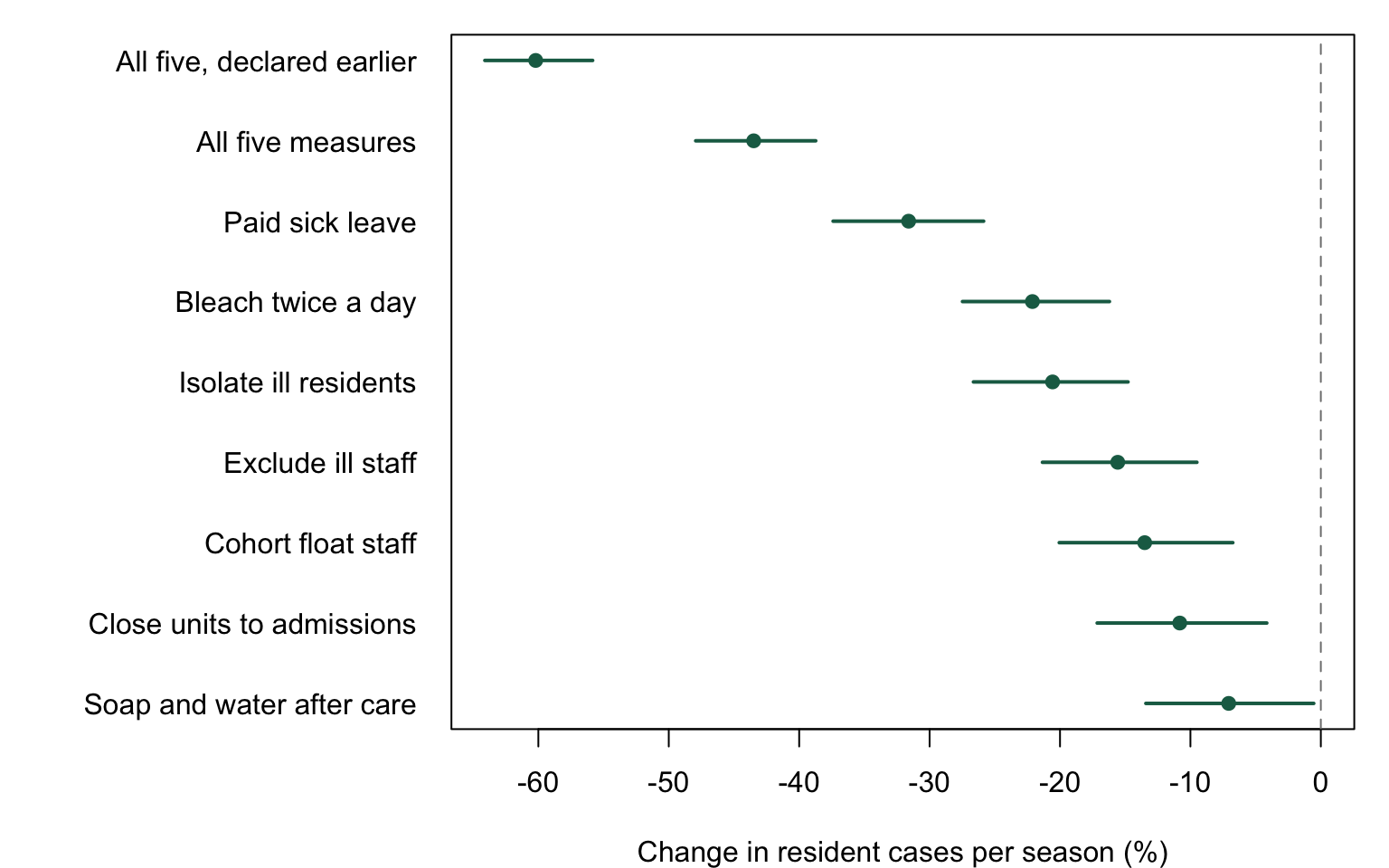
With no measures the facility averages 233 resident cases per 100 facility-seasons. Paid sick leave prevents the most of any single policy, 32% (95% interval 26 to 37), because it is the only one that acts before an outbreak is declared: with fewer ill staff at work, fewer staff introductions start outbreaks at all (10.5 against 13.3 outbreaks per 100 facility-seasons), in line with the 62% lower outbreak risk in New York nursing homes with paid sick leave (Li et al. 1996). Among the outbreak measures, hypochlorite cleaning twice a day prevents 22% (95% interval 16 to 27) and isolating ill residents 21% (95% interval 15 to 27), followed by excluding ill staff, 16% (95% interval 10 to 21), cohorting float staff, 14% (95% interval 7 to 20), and closing affected units to admissions, 11% (95% interval 4 to 17). Closure works by deferring admissions until the outbreak is over, so the residents who would have arrived during it are not exposed. Several of these intervals overlap, and Part 3 shows that the order of cleaning and isolation depends on a parameter the outbreak data do not fix. The five together prevent 43% (95% interval 39 to 48), and the same five declared after two cases with no reporting delay prevent 60% (95% interval 56 to 64): acting a day or two sooner adds 17 percentage points, close to the effect of the best single measure. This is the one result with field support, from Dutch nursing homes in which measures within three days of the first case were followed by lower staff attack rates (Friesema et al. 2009) and Australian ones in which prompt notification was followed by shorter outbreaks (Davis et al. 2011).
Excluding ill staff has a cost the case counts do not show: keeping staff home for 48 hours after their symptoms end raises staff shifts lost from 145 to 284 per 100 facility-seasons. Paid sick leave loses fewer shifts (138) because it prevents outbreaks and with them the staff cases. The bundle produces more declared outbreaks than no measures (15.1 against 13.3 per 100 facility-seasons) most likely because outbreaks it stops early can resume after the 14-day window and count again; the median outbreak falls from 21 to 11 cases.
Hand hygiene: what a model can and cannot say
hh_pct <- sapply(hh_runs, function(r) pct_change(r, base))
round(hh_pct, 1)
0.95 0.8 0.5
est 0.5 -7.1 -12.4
lo -4.0 -13.4 -19.0
hi 5.1 -0.5 -5.5Washing with soap and water after care, rather than using alcohol hand rub, prevents 7% of resident cases in the model when it cuts what staff hands carry by 20% (95% interval 0 to 13) and 12% when it cuts it by half; a 5% cut has no detectable effect (95% interval -4% to 5% change). The per-contact effect is an assumption, and the evidence on it points in different directions. In the laboratory, soap and water removes more norovirus from fingers than alcohol rub (Tuladhar et al. 2015). In the field, facilities whose staff preferred alcohol rub had six times the odds of an outbreak (adjusted odds ratio 6.06, 95% CI 1.44 to 33.99; Blaney et al. 2011), but a cluster-randomized trial of a hand hygiene program in 33 Dutch nursing homes found no reduction in gastroenteritis (Teesing et al. 2021). A compartmental model in which staff hands carry most transmission found that raising staff hand hygiene from 15% to 60% compliance cut cases by 75% (Assab and Temime 2016).
The model cannot settle this, and it shows why. Hand hygiene can only act on the transmission that passes through hands, and how much does is a structural choice. Here hands act through care contact and through staff contact with surfaces, but staff who are not infected do not carry virus from one resident to the next, and most residents are infected by other residents in shared spaces; so even a large per-contact effect does modestly for residents. A model that routes transmission through staff hands will find large effects; one that routes it elsewhere will find small ones; both can reproduce the same outbreaks. What the model can say is what it would take to observe an effect. With the season-to-season variation in this model, a two-arm study would need about 15,042 facility-seasons per arm to detect a 10% reduction in resident cases with 80% power, and about 1,671 to detect a 30% reduction. The trial that found nothing followed 33 homes for 13 months. Absence of a detected effect in the field and a large effect in a model are both consistent with a modest true effect.
Part 3: The Same Outbreaks, Different Routes
Parts 1 and 2 used a calibration in which 30% of transmission runs through the environment. Nothing in the outbreak data fixes that number. Part 3 sets it to 10%, 20%, 45%, and 60% instead, rescales beta and env.dep at each so that the model reproduces the same outbreaks, and reruns the baseline and five of the scenarios.
ridge_arms <- c("isolate", "exclude", "cohort", "clean", "bundle")
ridge <- lapply(seq_len(nrow(calib)), function(k) {
  if (k == central) return(c(list(none = base), runs[ridge_arms]))
  cal <- list(beta = calib$beta[k], env.dep = calib$env.dep[k])
  out <- list(none = run_scenario(cal, nsims))
  for (a in ridge_arms) out[[a]] <- run_scenario(c(cal, arms[[a]]), nsims)
  out
})
# Each calibration against the outbreak targets.
ridge_fit <- do.call(rbind, lapply(seq_along(ridge), function(k) {
r <- ridge[[k]]$none
s <- ob_stats(r)
data.frame(
calibration = k, beta = calib$beta[k], env.dep = calib$env.dep[k],
env_share = 100 * env_share(r),
outbreaks = 100 * r$tot$weight[1] * mean(r$tot$outbreaks),
res_cases = per100(r, "res_cases")[["mean"]],
size = med_iqr(s$size), ar_res = med_iqr(s$ar_res, pct = TRUE),
days = med_iqr(s$days)
)
}))knitr::kable(
data.frame(Calibration = ridge_fit$calibration, beta = ridge_fit$beta,
env.dep = ridge_fit$env.dep,
`Environmental share (%)` = round(ridge_fit$env_share),
Outbreaks = round(ridge_fit$outbreaks, 1),
`Resident cases` = round(ridge_fit$res_cases),
`Cases per outbreak` = ridge_fit$size,
`Resident attack rate (%)` = ridge_fit$ar_res,
`Duration (days)` = ridge_fit$days, check.names = FALSE),
align = "rrrrrrrrr")| Calibration | beta | env.dep | Environmental share (%) | Outbreaks | Resident cases | Cases per outbreak | Resident attack rate (%) | Duration (days) |
|---|---|---|---|---|---|---|---|---|
| 1 | 0.935 | 0.0520 | 11 | 12.9 | 210 | 21 [16, 28] | 38 [28, 47] | 15 [11, 23] |
| 2 | 0.796 | 0.1010 | 21 | 14.0 | 223 | 22 [15, 27] | 36 [25, 44] | 15 [11, 24] |
| 3 | 0.670 | 0.1485 | 31 | 13.3 | 233 | 21 [17, 32] | 38 [30, 47] | 16 [12, 26] |
| 4 | 0.490 | 0.2205 | 46 | 13.3 | 213 | 20 [15, 26] | 38 [28, 44] | 15 [11, 23] |
| 5 | 0.317 | 0.2894 | 61 | 13.3 | 226 | 21 [15, 28] | 38 [28, 47] | 16 [12, 23] |
The five calibrations are indistinguishable in the data used to set them: 12.9 to 14.0 outbreaks per 100 facility-seasons, 210 to 233 resident cases, the same median outbreak size, attack rate, and duration, and the same average epidemic curve to within simulation noise.
# The average outbreak, day by day from its first case, in each calibration.
ridge_cols <- c("#2a78d6", "#3b72a3", "#7f8e9c", "#c98a45", "#a8692a")
par(mfrow = c(1, 1), mar = c(4, 4.5, 1, 1))
curves <- lapply(ridge, function(x) {
  if (is.null(x$none$curves)) rep(NA, 40) else colMeans(x$none$curves, na.rm = TRUE)
})
ymax <- max(unlist(curves), 1, na.rm = TRUE)
plot(NA, xlim = c(0, 39), ylim = c(0, ymax * 1.05), xlab = "Days from the first case",
     ylab = "Symptom onsets per day, mean per outbreak")
for (k in seq_along(curves)) {
  if (all(is.na(curves[[k]]))) next
  lines(0:39, curves[[k]], col = ridge_cols[k], lwd = 2.5)
}
legend("topright", col = ridge_cols, lwd = 2.5, bty = "n",
       legend = sprintf("%.0f%% environmental", ridge_fit$env_share))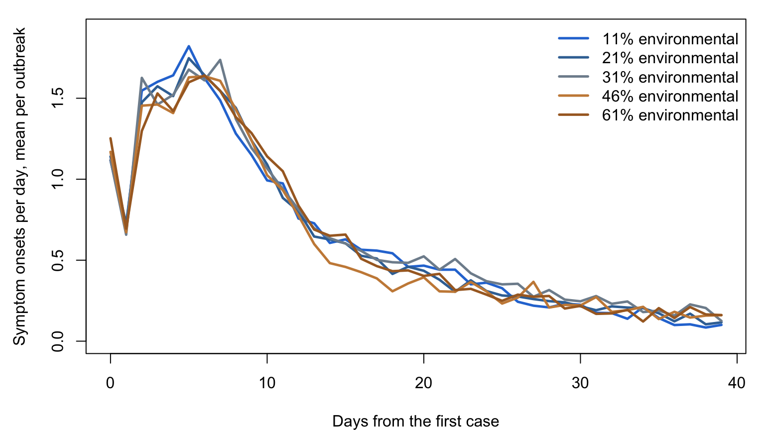
# How much each measure prevents, against the environmental share.
ridge_pct <- lapply(ridge_arms, function(a) {
  t(sapply(ridge, function(x) pct_change(x[[a]], x$none)))
})
names(ridge_pct) <- ridge_arms
arm_cols <- c(isolate = "#1a6b54", exclude = "#2a78d6", cohort = "#d9822b",
              clean = "#a8692a", bundle = "#46515b")
xs <- ridge_fit$env_share
par(mfrow = c(1, 1), mar = c(4, 4.5, 1, 1))
plot(NA, xlim = range(c(0, xs, 65), na.rm = TRUE),
     ylim = c(min(c(0, unlist(ridge_pct)), na.rm = TRUE) - 12, 0),
     xlab = "Share of transmission through the environment (%)",
     ylab = "Change in resident cases per season (%)")
abline(h = 0, lty = 2, col = "gray50")
for (a in ridge_arms) {
  m <- ridge_pct[[a]]
  polygon(c(xs, rev(xs)), c(m[, "lo"], rev(m[, "hi"])),
          col = adjustcolor(arm_cols[[a]], 0.15), border = NA)
  lines(xs, m[, "est"], col = arm_cols[[a]], lwd = 2.5, type = "b", pch = 19)
}
legend("bottom", col = arm_cols, lwd = 2.5, pch = 19, bty = "n", ncol = 3,
       legend = arm_lab[ridge_arms])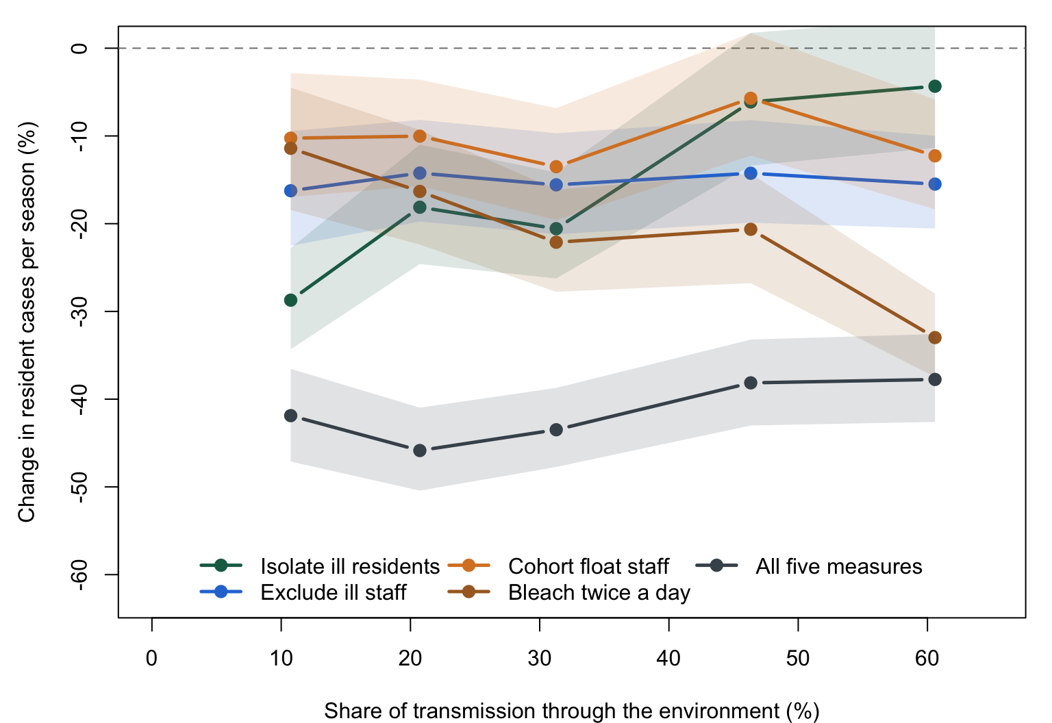
The measures do not respond alike. Isolating ill residents prevents 29% of resident cases when 11% of transmission is environmental and 4% when 61% is; hypochlorite cleaning prevents 11% and 33%. At the low end isolation ranks first and cleaning last; at the high end cleaning ranks first and isolation last, and the two cross near a 30% share, which is where the central calibration sits. Excluding ill staff prevents 14% to 16% at every share, because excluded staff neither infect people nor shed onto surfaces, and cohorting float staff varies between 6% and 14% without a trend. The five measures together prevent 38% to 46% across the five calibrations: a bundle that acts on both routes depends little on the split, and single measures depend on it heavily.
This is a practical identifiability problem of a kind described for cholera, where direct and waterborne transmission are identifiable in principle but, with noisy case data, only a combination of the waterborne parameters can be estimated (Eisenberg et al. 2013), and for a vector-borne model in which the reproduction number was recovered across the unidentifiable range while predicted intervention effects were wrong (Kao and Eisenberg 2018). When structurally different cholera models were fitted to the same epidemic data, every one of them fit (Lee et al. 2017). A model of norovirus calibrated only to outbreak counts and attack rates can rank isolation and cleaning in either order, and the ranking reflects the modeler’s assumption about the environment rather than the data.
How hard the routes are to tell apart also depends on how the environment is built. Here each reservoir is shared by a whole unit, like the dining-room contact it competes with, and with routine cleaning it loses half its contamination in about 1.3 days, well under the 3.6-day serial interval. The reservoir therefore acts like unit-wide contact with a short delay, which is the case the theory identifies as hardest to separate (Tien and Earn 2010). Reservoirs for each room, or surfaces that hold infectious virus for longer, would give the environmental route more of a signature of its own in the timing of cases.
What would separate the routes
The same figure shows what would. The measures respond in opposite directions to the share, so data on outbreaks under different measures carry information that outbreak counts do not:
- Timing relative to cleaning. Cleaning at known times is an input whose effect depends on the environmental share; a time-varying input of this kind cannot make the parameters less identifiable and can make them identifiable (Conrad et al. 2026). Onsets in the days after hypochlorite cleaning begins, compared with onsets after isolation begins, carry the signal.
- Variation across facilities. Facilities that respond with different measures, or with the same measures in a different order, are a natural experiment, as in the comparison of 72-hour and 48-hour staff exclusion across English counties (Vivancos et al. 2010); pooling many small outbreaks in one model estimates how transmission varies with facility characteristics (O’Dea et al. 2014).
- Measurements of the reservoir. Measuring how much virus the reservoir holds, and how long it lasts, restored identifiability in the cholera analysis. Environmental swabs in long-term care outbreaks find norovirus on resident room surfaces, dining tables, and a staff-only elevator button two weeks into an outbreak, with sequences identical to the cases’ (Wu et al. 2005); swab data become a calibration target once a model links surface concentration to risk.
- Genomes. Sequences that link cases with no contact in common point to an environmental source (Brown et al. 2019).
Next Steps
- Toward an enteric model family. The reservoir module is the start of a person-place layer: places with a membership that changes by shift, deposition and pickup by time spent, decay, and cleaning on a schedule. Generalizing it to rooms and shared bathrooms, hands as a second compartment, and places shared across facilities would serve norovirus, Clostridioides difficile, and other environmentally transmitted pathogens.
- Calibration to an outbreak line list with environmental swabs, the design Part 3 suggests, using the onset times of residents and staff and the dates each measure began.
- More than one facility. Staff who work in more than one nursing home connected facilities in the US during COVID-19 (Chen et al. 2021); hospital transfers connect facilities as well. A regional model would add facilities as groups and staff with two workplaces.
- Vaccination. No norovirus vaccine is licensed, and the leading candidate for adults did not meet its early efficacy threshold in 2026. A resident or staff vaccine arm, with efficacy in the range seen in young adults, is a straightforward extension once a product’s effect in older adults is known.
References
Burden, outbreak characteristics, and control:
- Calderwood LE, Wikswo ME, Mattison CP, et al. (2022). Norovirus outbreaks in long-term care facilities in the United States, 2009-2018: a decade of surveillance. Clin Infect Dis 74(1):113-119. https://doi.org/10.1093/cid/ciab808
- Calderwood L, Mirza S. (2026). Changes to trends in reported long-term care norovirus outbreaks in the United States during 2015-2025 (abstract). Antimicrob Steward Healthc Epidemiol 6(S1). https://doi.org/10.1017/ash.2026.10643
- Rosenthal NA, Lee LE, Vermeulen BAJ, et al. (2011). Epidemiological and genetic characteristics of norovirus outbreaks in long-term care facilities, 2003-2006. Epidemiol Infect 139(2):286-294. https://doi.org/10.1017/S095026881000083X
- Friesema IHM, Vennema H, Heijne JCM, et al. (2009). Norovirus outbreaks in nursing homes: the evaluation of infection control measures. Epidemiol Infect 137(12):1722-1733. https://doi.org/10.1017/S095026880900274X
- Inns T, Clough HE, Harris JP, et al. (2019). Estimating the burden of care home gastroenteritis outbreaks in England, 2014-2016. BMC Infect Dis 19:12. https://doi.org/10.1186/s12879-018-3642-3
- Centers for Disease Control and Prevention. Norovirus facts and stats (accessed November 2026). https://www.cdc.gov/norovirus/data-research/
- Davis CA, Vally H, Beard FH. (2011). Norovirus in residential care facilities: does prompt notification of outbreaks help? Commun Dis Intell Q Rep 35(2):162-167. https://doi.org/10.33321/cdi.2011.35.12
- Harris JP, Lopman BA, O’Brien SJ. (2010). Infection control measures for norovirus: a systematic review of outbreaks in semi-enclosed settings. J Hosp Infect 74(1):1-9. https://doi.org/10.1016/j.jhin.2009.07.025
- Adams C, Peterson SR, Hall AJ, Parashar U, Lopman BA. (2022). Associations of infection control measures and norovirus outbreak outcomes in healthcare settings: a systematic review and meta-analysis. Expert Rev Anti Infect Ther 20(2):279-290. https://doi.org/10.1080/14787210.2021.1949985
- MacCannell T, Umscheid CA, Agarwal RK, et al. (2011). Guideline for the prevention and control of norovirus gastroenteritis outbreaks in healthcare settings. Infect Control Hosp Epidemiol 32(10):939-969. https://doi.org/10.1086/662025
- Li J, Birkhead GS, Strogatz DS, Coles FB. (1996). Impact of institution size, staffing patterns, and infection control practices on communicable disease outbreaks in New York State nursing homes. Am J Epidemiol 143(10):1042-1049. https://doi.org/10.1093/oxfordjournals.aje.a008668
- Chiu S, Black CL, Yue X, et al. (2017). Working with influenza-like illness: presenteeism among US health care personnel during the 2014-2015 influenza season. Am J Infect Control 45(11):1254-1258. https://doi.org/10.1016/j.ajic.2017.04.008
- Vivancos R, Sundkvist T, Barker D, Burton J, Nair P. (2010). Effect of exclusion policy on the control of outbreaks of suspected viral gastroenteritis: analysis of outbreak investigations in care homes. Am J Infect Control 38(2):139-143. https://doi.org/10.1016/j.ajic.2009.02.011
- Blaney DD, Daly ER, Kirkland KB, et al. (2011). Use of alcohol-based hand sanitizers as a risk factor for norovirus outbreaks in long-term care facilities in northern New England: December 2006 to March 2007. Am J Infect Control 39(4):296-301. https://doi.org/10.1016/j.ajic.2010.10.010
- Teesing GR, Richardus JH, Nieboer D, et al. (2021). The effect of a hand hygiene intervention on infections in residents of nursing homes: a cluster randomized controlled trial. Antimicrob Resist Infect Control 10:80. https://doi.org/10.1186/s13756-021-00946-3
- Tuladhar E, Hazeleger WC, Koopmans M, et al. (2015). Reducing viral contamination from finger pads: handwashing is more effective than alcohol-based hand disinfectants. J Hosp Infect 90(3):226-234. https://doi.org/10.1016/j.jhin.2015.02.019
Natural history and transmission:
- Centers for Disease Control and Prevention. (2011). Updated norovirus outbreak management and disease prevention guidelines. MMWR Recomm Rep 60(RR-3):1-18. PMID 21368741.
- Lee RM, Lessler J, Lee RA, et al. (2013). Incubation periods of viral gastroenteritis: a systematic review. BMC Infect Dis 13:446. https://doi.org/10.1186/1471-2334-13-446
- Lopman BA, Reacher MH, Vipond IB, Sarangi J, Brown DWG. (2004). Clinical manifestation of norovirus gastroenteritis in health care settings. Clin Infect Dis 39(3):318-324. https://doi.org/10.1086/421948
- Teunis PFM, Sukhrie FHA, Vennema H, et al. (2015). Shedding of norovirus in symptomatic and asymptomatic infections. Epidemiol Infect 143(8):1710-1717. https://doi.org/10.1017/S095026881400274X
- Simmons K, Gambhir M, Leon J, Lopman B. (2013). Duration of immunity to norovirus gastroenteritis. Emerg Infect Dis 19(8):1260-1267. https://doi.org/10.3201/eid1908.130472
- Thorvén M, Grahn A, Hedlund KO, et al. (2005). A homozygous nonsense mutation (428G to A) in the human secretor (FUT2) gene provides resistance to symptomatic norovirus (GGII) infections. J Virol 79(24):15351-15355. https://doi.org/10.1128/JVI.79.24.15351-15355.2005
- Kirby AE, Streby A, Moe CL. (2016). Vomiting as a symptom and transmission risk in norovirus illness: evidence from human challenge studies. PLoS One 11(4):e0143759. https://doi.org/10.1371/journal.pone.0143759
- Adams C, Young D, Gastañaduy PA, et al. (2020). Quantifying the roles of vomiting, diarrhea, and residents vs. staff in norovirus transmission in U.S. nursing home outbreaks. PLoS Comput Biol 16(3):e1007271. https://doi.org/10.1371/journal.pcbi.1007271
- Chen Y, Lopman BA, Hall AJ, et al. (2023). Factors driving norovirus transmission in long-term care facilities: a case-level analysis of 107 outbreaks. Epidemics 42:100671. https://doi.org/10.1016/j.epidem.2023.100671
- Sukhrie FHA, Teunis P, Vennema H, et al. (2012). Nosocomial transmission of norovirus is mainly caused by symptomatic cases. Clin Infect Dis 54(7):931-937. https://doi.org/10.1093/cid/cir971
- Heijne JCM, Rondy M, Verhoef L, et al. (2012). Quantifying transmission of norovirus during an outbreak. Epidemiology 23(2):277-284. https://doi.org/10.1097/EDE.0b013e3182456ee6
The environment and identifiability:
- Lopman B, Gastañaduy P, Park GW, et al. (2012). Environmental transmission of norovirus gastroenteritis. Curr Opin Virol 2(1):96-102. https://doi.org/10.1016/j.coviro.2011.11.005
- Li S, Eisenberg JNS, Spicknall IH, Koopman JS. (2009). Dynamics and control of infections transmitted from person to person through the environment. Am J Epidemiol 170(2):257-265. https://doi.org/10.1093/aje/kwp116
- Kraay ANM, Hayashi MAL, Hernandez-Ceron N, et al. (2018). Fomite-mediated transmission as a sufficient pathway: a comparative analysis across three viral pathogens. BMC Infect Dis 18:540. https://doi.org/10.1186/s12879-018-3425-x
- Kim AN, Park SY, Bae SC, Oh MH, Ha SD. (2014). Survival of norovirus surrogate on various food-contact surfaces. Food Environ Virol 6(3):182-188. https://doi.org/10.1007/s12560-014-9154-4
- Fallahi S, Mattison K. (2011). Evaluation of murine norovirus persistence in environments relevant to food production and processing. J Food Prot 74(11):1847-1851. https://doi.org/10.4315/0362-028X.JFP-11-081
- Barker J, Vipond IB, Bloomfield SF. (2004). Effects of cleaning and disinfection in reducing the spread of norovirus contamination via environmental surfaces. J Hosp Infect 58(1):42-49. https://doi.org/10.1016/j.jhin.2004.04.021
- Wu HM, Fornek M, Schwab KJ, et al. (2005). A norovirus outbreak at a long-term-care facility: the role of environmental surface contamination. Infect Control Hosp Epidemiol 26(10):802-810. https://doi.org/10.1086/502497
- Tien JH, Earn DJD. (2010). Multiple transmission pathways and disease dynamics in a waterborne pathogen model. Bull Math Biol 72(6):1506-1533. https://doi.org/10.1007/s11538-010-9507-6
- Eisenberg MC, Robertson SL, Tien JH. (2013). Identifiability and estimation of multiple transmission pathways in cholera and waterborne disease. J Theor Biol 324:84-102. https://doi.org/10.1016/j.jtbi.2012.12.021
- Kao YH, Eisenberg MC. (2018). Practical unidentifiability of a simple vector-borne disease model: implications for parameter estimation and intervention assessment. Epidemics 25:89-100. https://doi.org/10.1016/j.epidem.2018.05.010
- Lee EC, Kelly MR, Ochocki BM, et al. (2017). Model distinguishability and inference robustness in mechanisms of cholera transmission and loss of immunity. J Theor Biol 420:68-81. https://doi.org/10.1016/j.jtbi.2017.01.032
- Conrad JR, Hyman JM, Eisenberg MC. (2026). Examining the impact of forcing function inputs on structural identifiability. Math Biosci 402:109814. https://doi.org/10.1016/j.mbs.2026.109814
- O’Dea EB, Pepin KM, Lopman BA, Wilke CO. (2014). Fitting outbreak models to data from many small norovirus outbreaks. Epidemics 6:18-29. https://doi.org/10.1016/j.epidem.2013.12.002
- Brown JR, Roy S, Shah D, et al. (2019). Norovirus transmission dynamics in a pediatric hospital using full genome sequences. Clin Infect Dis 68(2):222-228. https://doi.org/10.1093/cid/ciy438
Other models and the facility:
- Gaythorpe KAM, Trotter CL, Lopman B, Steele M, Conlan AJK. (2018). Norovirus transmission dynamics: a modelling review. Epidemiol Infect 146(2):147-158. https://doi.org/10.1017/S0950268817002692
- Towers S, Chen J, Cruz C, et al. (2018). Quantifying the relative effects of environmental and direct transmission of norovirus. R Soc Open Sci 5(3):170602. https://doi.org/10.1098/rsos.170602
- Assab R, Temime L. (2016). The role of hand hygiene in controlling norovirus spread in nursing homes. BMC Infect Dis 16:395. https://doi.org/10.1186/s12879-016-1702-0
- Rushton SP, Sanderson RA, Reid WDK, et al. (2019). Transmission routes of rare seasonal diseases: the case of norovirus infections. Philos Trans R Soc B 374(1776):20180267. https://doi.org/10.1098/rstb.2018.0267
- Duval A, Obadia T, Martinet L, et al. (2018). Measuring dynamic social contacts in a rehabilitation hospital: effect of wards, patient and staff characteristics. Sci Rep 8:1686. https://doi.org/10.1038/s41598-018-20008-w
- Champredon D, Najafi M, Laskowski M, Chit A, Moghadas SM. (2018). Individual movements and contact patterns in a Canadian long-term care facility. AIMS Public Health 5(2):111-121. https://doi.org/10.3934/publichealth.2018.2.111
- Zhu X, et al. (2022). Nursing home design and COVID-19: implications for guidelines and regulation. J Am Med Dir Assoc 23(2):272-279. https://doi.org/10.1016/j.jamda.2021.12.026
- Parrón I, Álvarez J, Jané M, et al. (2019). A foodborne norovirus outbreak in a nursing home and spread to staff and their household contacts. Epidemiol Infect 147:e225. https://doi.org/10.1017/S0950268819001146
- Chen MK, Chevalier JA, Long EF. (2021). Nursing home staff networks and COVID-19. Proc Natl Acad Sci U S A 118(1):e2015455118. https://doi.org/10.1073/pnas.2015455118
Facility size, staffing, and turnover are from Centers for Medicare and Medicaid Services public files (Provider Information, October 2026; Payroll-Based Journal, second quarter of 2026; skilled nursing facility cost reports, fiscal year 2023). The contact weights, the cleaning fractions, the precaution and hand hygiene multipliers, and the split of introductions between staff and admissions are illustrative. The two transmission parameters and the introduction rate were set to reproduce published outbreak sizes and frequency; the model is not calibrated to any facility’s data.