flowchart LR
    S["<b>S</b>"] -->|"contact hours<br/>(se.flow)"| E
    E["<b>E</b><br/>incubating"] -->|"incubation drawn<br/>at infection"| I
    I["<b>I</b><br/>one week"] -->|"death<br/>(id.flow)"| D["<b>D</b>"]
    S -.->|"vax.cov<br/>at baseline"| R["<b>R</b>"]

    style S fill:#3498db,color:#fff
    style E fill:#8e44ad,color:#fff
    style I fill:#e74c3c,color:#fff
    style D fill:#7f8c8d,color:#fff
    style R fill:#27ae60,color:#fff
Rabies on an Observed Raccoon Contact Network
SEI
zoonotic
rabies
wildlife
observed network
netcensus
intermediate
A zoonotic pathogen simulated over an empirical wildlife network. Weekly proximity-logger contacts among 24 suburban adult raccoons (Hirsch et al. 2013; Reynolds et al. 2015) enter netsim as a netcensus layer with no ERGM; the example asks how the time of year of a hypothetical rabies introduction and the share of raccoons immune change the size of an outbreak.
Overview
Most Gallery examples estimate a network model from summary statistics and simulate from it. This one does not. Hirsch et al. (2013) fitted proximity-logging collars to nearly all the resident adult raccoons (Procyon lotor) in a 20-ha core of a suburban forest preserve in Cook County, Illinois, and Reynolds et al. (2015) deposited 52 weekly matrices of contact time among 24 of them. For those animals there is nothing to estimate: the network goes into netsim as it is, through netcensus(), and the simulation reads the contacts of week at at time step at.
It is a record of collared adults, not of the whole population. The core area is part of a 1,499-ha preserve with 40 to 70 raccoons per km², kits are too small to collar, and collars failed and were replaced through the year, so a raccoon with no recorded contact in a week may simply have had a collar that was not working (Hirsch et al. 2013). The simulation treats the recorded network as the whole contact structure, so its outbreaks are outbreaks among these adults; the page comes back to what that leaves out.
Hirsch et al. collared these raccoons to study the potential for pathogen transmission in general, naming rabies, canine distemper, parvovirus, and leptospirosis, and noted that proximity collars reflect pathogens spread by close contact better than rabies, which is spread by bites. Rabies is the pathogen here because Reynolds et al. (2015) simulated it on these data and because the raccoon is its main terrestrial reservoir in the eastern United States, where oral rabies vaccination (ORV) is the main control and a vaccination barrier is maintained to stop the raccoon variant from spreading west (Elmore et al. 2017). Illinois lies west of that barrier, so every introduction in this example is hypothetical. The questions are close to the source paper’s: how much does the time of year of an introduction matter, and how much immunity does it take to keep an outbreak small? The example combines four things:
An observed dynamic network as the contact layer.
netcensus()wraps anetworkDynamicobject built from the weekly contact matrices. No formation model, no dissolution model, nonetdx. At each step the network module reads that week’s contacts from the census instead of simulating them, so the layer works with EpiModel’s built-in models as well as with custom modules.Contact intensity from the data, through an assumption. The census layer records who was in contact; the hours of contact for each pair and week go to the infection module as a parameter, and the per-pair transmission probability is a constant hazard per hour of proximity. Rabies is spread by bites, so proximity time stands in for the opportunity to bite, and the page treats what follows from it as consequences of that assumption.
A rabies natural history without recovery. Susceptible, incubating for a period drawn at infection, infectious for one week, dead. Death does not remove a raccoon from the census (the node set is fixed); it makes it inert.
Introduction timing and immunity. One infectious raccoon is introduced in a week drawn at random for each simulation, so a single
netsim()call covers the whole year, into a population with 0, 25, 50, or 75 percent of raccoons immune at baseline. The outcome is the number of additional cases.
NoteWhere this sits among wildlife network methods
The animal social network literature has its own toolkit for building and comparing contact networks from proximity, association, and telemetry data (Farine and Whitehead 2015), and epidemic simulation over those observed networks is common, including with EpiModel (Webber et al. 2016 predicted pathogen transmission over the roosting networks of big brown bat colonies). What netcensus() adds is the plumbing: the observed network becomes an ordinary netsim layer, so the built-in disease types, the transmission matrix, the module API, and multi-layer models are all available on it without custom initialization or infection code. The other route from observed animal networks into EpiModel is to fit an ERGM or TERGM to them and simulate from the fit, which generalizes beyond the observed animals and is the right choice when the observed network is a sample of a larger population, as this one partly is.
TipDownload standalone scripts
- model.R - Main simulation script
- module-fx.R - Custom module functions
- raccoon_contacts.csv - Weekly contact seconds between raccoon pairs
Model Structure
| Status | Description |
|---|---|
s |
Susceptible |
e |
Exposed: infected and incubating, not infectious |
i |
Infectious: clinical rabies, transmits for one week, then dies |
d |
Dead of rabies |
r |
Immune at baseline (vaccinated) |
The time step is one week, the resolution of the contact data. Each infected raccoon draws an incubation period at infection, the number of weeks until the week in which it is infectious; in that week it transmits, and it dies at the end of it. Rabies has a case fatality of one. Immunity is set once, at baseline, for a random set of raccoons.
Setup
suppressMessages(library(EpiModel))

nsims.week <- 100
ncores <- 5
intro.weeks <- 2:52
vax.covs <- c(0, 0.25, 0.5, 0.75)
nsteps <- 104
set.seed(2015)
These are the full settings of the standalone model.R: introductions in every week from 2 to 52 (modules first run at step 2, so week 1 cannot be one), about 100 simulations per week, and four levels of baseline immunity, about seven minutes on five cores. Run non-interactively, it drops to four introduction weeks, about five simulations per week, and two levels of immunity. The observed year is played twice, so nsteps is 104; the reason is below.
source("module-fx.R")The Observed Contact Network
Contacts were logged when two collared raccoons were within 1 to 1.5 m (Hirsch et al. 2013), and contacts under one second were excluded. raccoon_contacts.csv holds the 52 weekly matrices in long form, from the Animal Social Network Repository copy of the deposit: one row per pair and week with at least one contact, with the contact time in seconds. Raccoon ids run 1 to 24. The collared population was largest in July 2004, and the mating season in this population runs from December to March (Hirsch et al. 2013); with the deposit’s breeding season at weeks 24 to 39, week 1 falls in early July. The page groups the weeks into four 13-week seasons on that calendar.
contacts.raw <- read.csv("raccoon_contacts.csv")
stopifnot(all(contacts.raw$raccoon1 < contacts.raw$raccoon2))
n <- 24

cat(sprintf("%d pair-weeks of contact among %d raccoons over %d weeks\n",
            nrow(contacts.raw), n, max(contacts.raw$week)))
1997 pair-weeks of contact among 24 raccoons over 52 weeksWhat the collars recorded
A raccoon with no row in a week has no recorded contact that week. Most often its collar was not working: the network shrank over the study “mostly as a result of collar failure”, and raccoons were re-trapped to replace malfunctioning collars (Hirsch et al. 2013). Counting raccoons recorded, pairs in contact, and hours per pair separately keeps the collars apart from the behavior.
wk <- split(contacts.raw, factor(contacts.raw$week, levels = 1:52))
weekly <- data.frame(week = 1:52,
                     animals = sapply(wk, function(d) length(unique(c(d$raccoon1, d$raccoon2)))),
                     pairs = sapply(wk, nrow),
                     hours = sapply(wk, function(d) sum(d$seconds) / 3600))
weekly$hours.per.pair <- weekly$hours / weekly$pairs
weekly$density <- weekly$pairs / choose(weekly$animals, 2)

season.of <- function(week) {
  cut(week, c(0, 13, 26, 39, 52),
      labels = c("summer (Jul-Sep)", "autumn (Oct-Dec)",
                 "winter (Jan-Mar)", "spring (Apr-Jun)"))
}
data.season <- round(sapply(weekly[, c("animals", "pairs", "density", "hours.per.pair")],
                            function(x) tapply(x, season.of(weekly$week), mean)), 2)
knitr::kable(data.season, caption = "Weekly means by season: raccoons with any recorded contact, pairs in contact, share of the possible pairs among recorded raccoons that were in contact, and contact hours per pair in contact.")| animals | pairs | density | hours.per.pair | |
|---|---|---|---|---|
| summer (Jul-Sep) | 21.31 | 62.23 | 0.29 | 1.02 |
| autumn (Oct-Dec) | 16.23 | 37.08 | 0.30 | 7.95 |
| winter (Jan-Mar) | 12.92 | 24.08 | 0.34 | 10.75 |
| spring (Apr-Jun) | 14.54 | 30.23 | 0.31 | 3.09 |
par(mfrow = c(1, 3), mar = c(4, 4, 2, 1))
labs <- c(animals = "Raccoons recorded", pairs = "Pairs in contact",
          hours.per.pair = "Hours per pair in contact")
for (v in names(labs)) {
  y <- weekly[[v]]
  plot(1:52, y, type = "h", lwd = 3, col = "gray40", xlab = "Week",
       ylab = labs[v], main = labs[v], ylim = c(0, max(y)))
  rect(24, 0, 39, max(y) * 1.1, col = adjustcolor("orange", 0.2), border = NA)
}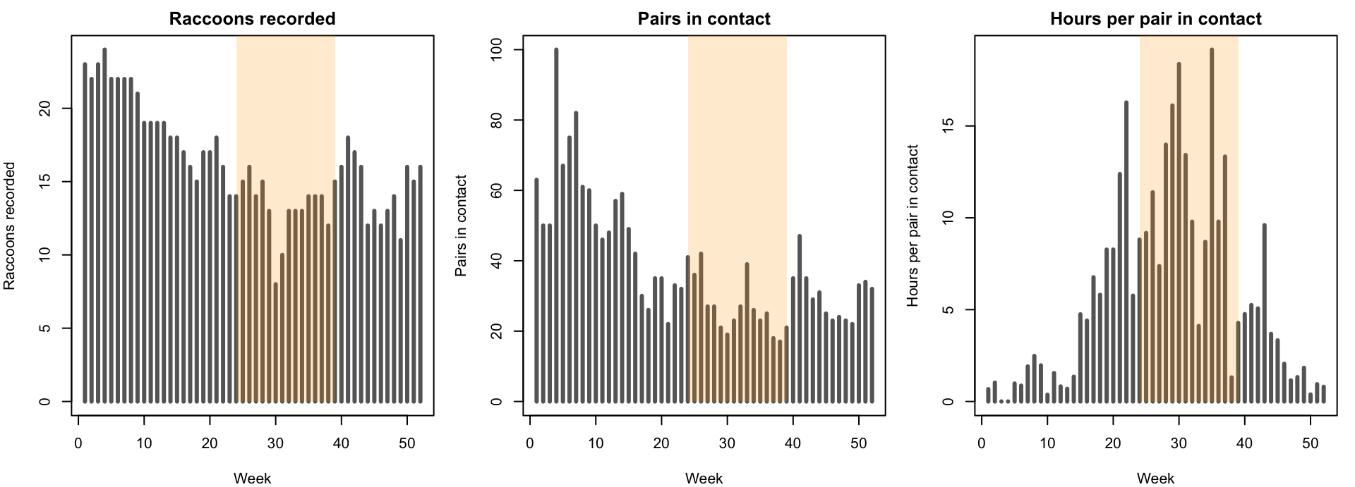
The number of pairs in contact follows the number of raccoons recorded (correlation 0.85), and the share of the possible pairs among recorded raccoons that were in contact barely changes across the seasons (0.29 to 0.34). Fewer pairs in winter is mostly fewer working collars. What changes with the season is the time pairs spend together: hours per pair in contact rise from 1.02 in summer to 10.75 in winter, consistent with raccoons denning together in cold weather (Hirsch et al. 2013), which Hirsch et al. (2016) found to be the main driver of seasonal rabies in this population. Long contacts are not confined to winter: some pairs spent 25 to 140 hours a week together in August and again in April and May.
Collar gaps also run through the breeding season. Three raccoons recorded both before and after it have no contacts for 11 to 17 weeks within it, so the winter network is the least completely observed part of the year, and the simulations below probably understate transmission in winter.
Data problems
Three features of the deposit are not raccoon behavior. Weeks 3 and 4 record as many pairs as the weeks around them (week 4 the most of any week), but 0.18 and 0.28 contact hours in total and no contact longer than five minutes, against tens to hundreds of hours in the weeks on either side; week 4 is also the first week of one collar and the last of two others, which suggests a trapping or collar-servicing week. Weeks 19 and 20 are identical row for row. And three pair-weeks record exactly a full week, 604,800 seconds, together: two in December and January, when sharing a den for a week is plausible, and one in week 37, in March.
print(round(weekly[1:8, c("week", "animals", "pairs", "hours")], 2)) week animals pairs hours
1 1 23 63 42.29
2 2 22 50 51.27
3 3 23 50 0.18
4 4 24 100 0.28
5 5 22 67 65.47
6 6 22 75 64.67
7 7 22 82 156.62
8 8 22 61 151.17w19 <- contacts.raw[contacts.raw$week == 19, -1]
w20 <- contacts.raw[contacts.raw$week == 20, -1]
cat("Weeks 19 and 20 identical:",
isTRUE(all.equal(w19[order(w19$raccoon1, w19$raccoon2), ],
w20[order(w20$raccoon1, w20$raccoon2), ],
check.attributes = FALSE)), "\n")Weeks 19 and 20 identical: TRUE print(contacts.raw[contacts.raw$seconds == 7 * 24 * 3600, ], row.names = FALSE) week raccoon1 raccoon2 seconds
25 4 14 604800
30 11 12 604800
37 7 10 604800The Animal Social Network Repository copy has the same values, and we found no explanation for them in the published sources. We treat weeks 3 and 4 as missing and fill each from the nearest observed week, week 2 for week 3 and week 5 for week 4. Left as recorded, they would make an introduction in either week almost certain to go nowhere and would put a two-week pause in transmission into both years of the run. Weeks 19 and 20 and the full-week contacts are kept: they look like real contact data, even if one week is repeated.
contacts <- rbind(contacts.raw[!contacts.raw$week %in% c(3, 4), ],
                  transform(contacts.raw[contacts.raw$week == 2, ], week = 3),
                  transform(contacts.raw[contacts.raw$week == 5, ], week = 4))
contacts <- contacts[order(contacts$week, contacts$raccoon1, contacts$raccoon2), ]
Playing the year twice
The year is observed once, but a rabies chain started late in that year has not run its course by week 52: with an incubation period of a month or more, a year holds only a few generations. We therefore play the observed year again as year two, on the assumption that the seasonal contact pattern repeats. Raccoons whose records ended during year one do not come back: their collars failed for good, or they died or left, and replaying their early-year contacts would bring them back to life. Year two holds only the raccoons still recorded in week 52.
last.week <- sapply(1:n, function(i) {
  max(contacts$week[contacts$raccoon1 == i | contacts$raccoon2 == i])
})
stayers <- which(last.week == 52)
cat("Raccoons in year two:", length(stayers), "of", n, "\n")
Raccoons in year two: 16 of 24 year2 <- contacts[contacts$raccoon1 %in% stayers & contacts$raccoon2 %in% stayers, ]
contacts2 <- rbind(contacts, transform(year2, week = week + 52))The census layer
Each pair-week becomes an edge spell covering that week, so that netsim’s time step at reads the contacts of week at. The networkDynamic object goes to netcensus(), whose print method summarizes the observed edges over the window.
nw <- network_initialize(n)
nw <- set_vertex_attribute(nw, "id", 1:n)
nwd <- networkDynamic::networkDynamic(
  base.net = nw,
  edge.spells = data.frame(onset = contacts2$week,
                           terminus = contacts2$week + 1,
                           tail = contacts2$raccoon1,
                           head = contacts2$raccoon2),
  verbose = FALSE
)
nwd %n% "net.obs.period" <- list(observations = list(c(1, nsteps + 1)),
                                 mode = "discrete", time.increment = 1,
                                 time.unit = "week")

obs <- netcensus(nwd)
obs
EpiModel Observed Network Layer
=======================
Model class: netcensus
Network type: dynamic (networkDynamic)
Layer Summary
-----------------------
Nodes: 24
Observation window: [1, 105), time steps 1 to 104
Edges ever observed: 220
Edges active per step: min 11 , median 29.5 , max 82
Mean degree per step: 2.74
Vertex attributes: idThere is no netest and no netdx in this example: the network was observed, so there is no model whose fit could be checked. netdx() refuses a netcensus object for that reason.
The census layer works with EpiModel’s built-in models as it is. A quick check with the built-in SI model, a fixed transmission probability per contact, and two raccoons infected at the start:
sim_si <- netsim(obs, param.net(inf.prob = 0.1, act.rate = 1), init.net(i.num = 2),
                 control.net(type = "SI", nsims = 1, nsteps = 52, tergmLite = TRUE,
                             resimulate.network = TRUE, verbose = FALSE))
print(tail(as.data.frame(sim_si)[, c("time", "s.num", "i.num")], 1), row.names = FALSE)
time s.num i.num
52 3 21Everything below replaces the built-in modules with custom ones; nothing about the layer changes.
The census layer is binary: a pair is in contact this week or it is not. The hours of contact for each pair and week go to the infection module as a parameter, one named vector per week, with the smaller id first in each name so that the module can look a pair up whichever way round it comes.
contact.hours <- lapply(1:nsteps, function(w) {
  cw <- contacts2[contacts2$week == w, ]
  setNames(cw$seconds / 3600, paste(pmin(cw$raccoon1, cw$raccoon2),
                                    pmax(cw$raccoon1, cw$raccoon2), sep = "_"))
})
Modules
Four custom modules carry the rabies process; the network needs none. They are in module-fx.R.
Infection. discord_edgelist() returns the susceptible-infectious pairs in contact this week from the census layer. The module looks up each pair’s contact hours, stops if a census edge has none (the two inputs would disagree), and draws transmission with probability 1 - exp(-inf.hazard * hours). A raccoon infected by more than one infectious raccoon in the same week is infected once, by one of them drawn at random. Each new infection draws its incubation period, and each transmission is recorded with set_transmat() together with the pair’s contact hours.
del <- discord_edgelist(dat, at, network = 1, infstat = "i")
key <- paste(pmin(del$sus, del$inf), pmax(del$sus, del$inf), sep = "_")
hours <- contact.hours[[at]][key]
if (anyNA(hours)) {
  stop("census edges without contact hours at step ", at,
       ": the network and contact.hours disagree")
}
del$hours <- unname(hours)
del$transProb <- 1 - exp(-inf.hazard * del$hours)
transmit <- rbinom(nrow(del), 1, del$transProb)
del <- del[which(transmit == 1), , drop = FALSE]
del <- del[sample.int(nrow(del)), , drop = FALSE]
del <- del[!duplicated(del$sus), , drop = FALSE]
idsNewInf <- del$sus
incub[idsNewInf] <- pmax(1, round(rgamma(length(idsNewInf), shape = inc.shape,
                                         scale = inc.mean / inc.shape)))
Progression. A raccoon infected in week t with incubation period d is infectious in week t + d: it becomes i at the end of week t + d - 1, transmits in week t + d, and dies at the end of that week. Drawing the duration at infection, rather than leaving each week with a constant probability, gives the incubation period the shape of the observed one; a constant weekly probability makes one week the most common incubation period.
Introduction. Each simulation draws its introduction week from the candidate weeks at its first step and stores it with set_param(). This is a general pattern for a parameter that should vary between the simulations of one netsim() call; recording it with set_epi() puts it in the output next to the outcomes. In that week, one susceptible raccoon with at least one contact becomes infectious.
intro.week <- get_param(dat, "intro.week")
if (at == 2 && length(intro.week) > 1) {
  intro.week <- intro.week[sample.int(length(intro.week), 1)]
  dat <- set_param(dat, "intro.week", intro.week)
}
dat <- set_epi(dat, "intro.week", intro.week)
Vaccination. At step 2, round(vax.cov * 24) raccoons drawn at random are set to r. This is the share immune after baiting (seroprevalence), not the share of raccoons that took a bait.
Parameters
| Parameter | Value | Meaning |
|---|---|---|
inf.hazard |
0.5 per hour | Transmission hazard per hour of proximity. A three-minute contact in a week transmits with probability 0.02, an hour with 0.39, a day together with 1. An assumption: proximity stands in for bites. At this site raccoons interacted aggressively in 7% of interactions at feeding stations, and Hirsch et al. (2013) judged brief encounters unlikely to be enough for rabies. |
inc.mean, inc.shape |
6 weeks, 6 | Incubation period from infection to the infectious week, a gamma distribution rounded to whole weeks: mode 5 weeks (Tinline et al. 2002), 94% of draws between 3 and 12 weeks (Hirsch et al. 2013). |
| Infectious period | 1 week | Clinical rabies lasts days, and the infection window is about one week (Hirsch et al. 2013). The case dies at the end of its infectious week. |
intro.week |
2 to 52 | Candidate weeks for the introduction; each simulation draws one. |
vax.cov |
0, 0.25, 0.5, 0.75 | Share of the 24 raccoons immune at baseline (6, 12, and 18 animals). Post-baiting seroprevalence in raccoon ORV campaigns has mostly been 10% to 55%, and 67% to 78% in a few (Elmore et al. 2017, Table 1). |
param <- param.net(
  inf.hazard = 0.5,
  inc.mean = 6,
  inc.shape = 6,
  intro.week = intro.weeks,
  vax.cov = 0,
  contact.hours = contact.hours
)
init <- init.net(i.num = 0)
Every raccoon starts susceptible; the introduction module seeds the infection. The control settings name the custom modules and fix their order. The census layer needs no resimulation of its own, but under tergmLite the built-in resim_nets module is what reads the week’s contacts from the observed network, so it stays in the pipeline ahead of infection; resimulate.network = TRUE is what tergmLite requires, and setting it avoids a warning.
control <- control.net(
  type = NULL,
  nsims = nsims.week * length(intro.weeks),
  ncores = ncores,
  nsteps = nsteps,
  tergmLite = TRUE,
  resimulate.network = TRUE,
  vaccinate.FUN = vaccinate,
  introduce.FUN = introduce,
  infection.FUN = infect,
  progress.FUN = progress,
  prevalence.FUN = prevalence,
  module.order = c("vaccinate.FUN", "resim_nets.FUN", "summary_nets.FUN",
                   "introduce.FUN", "infection.FUN", "progress.FUN",
                   "nwupdate.FUN", "prevalence.FUN"),
  save.transmat = TRUE,
  save.nwstats = FALSE,
  verbose = FALSE
)
Transmission Potential from the Data
Before any simulation, the contact data and the hazard say how transmissible each week is. An infectious raccoon infects each of its contacts that week with probability 1 - exp(-inf.hazard * hours). For each raccoon in contact that week, the sum of those probabilities is the expected number it infects directly, and one minus the product of their complements is the probability that it infects at least one. Averaged over the raccoons in contact that week, which is how the introduction module picks the introduced animal, these are the expected direct infections and the chance of any onward transmission from an introduction in that week.
potential <- t(sapply(1:52, function(w) {
  cw <- contacts[contacts$week == w, ]
  p <- 1 - exp(-param$inf.hazard * cw$seconds / 3600)
  ids <- unique(c(cw$raccoon1, cw$raccoon2))
  mine <- lapply(ids, function(i) p[cw$raccoon1 == i | cw$raccoon2 == i])
  c(direct = mean(sapply(mine, sum)),
    any = mean(sapply(mine, function(q) 1 - prod(1 - q))))
}))par(mfrow = c(1, 1), mar = c(4, 4, 2, 1))
plot(1:52, potential[, "direct"], type = "h", lwd = 4, col = "gray40",
xlab = "Week", ylab = "Expected raccoons infected directly",
ylim = c(0, max(potential[, "direct"]) * 1.1))
rect(24, 0, 39, max(potential[, "direct"]) * 1.1, col = adjustcolor("orange", 0.2),
border = NA)
abline(h = 1, lty = 3, col = "gray50")
abline(v = c(13.5, 26.5, 39.5), lty = 2, col = "gray70")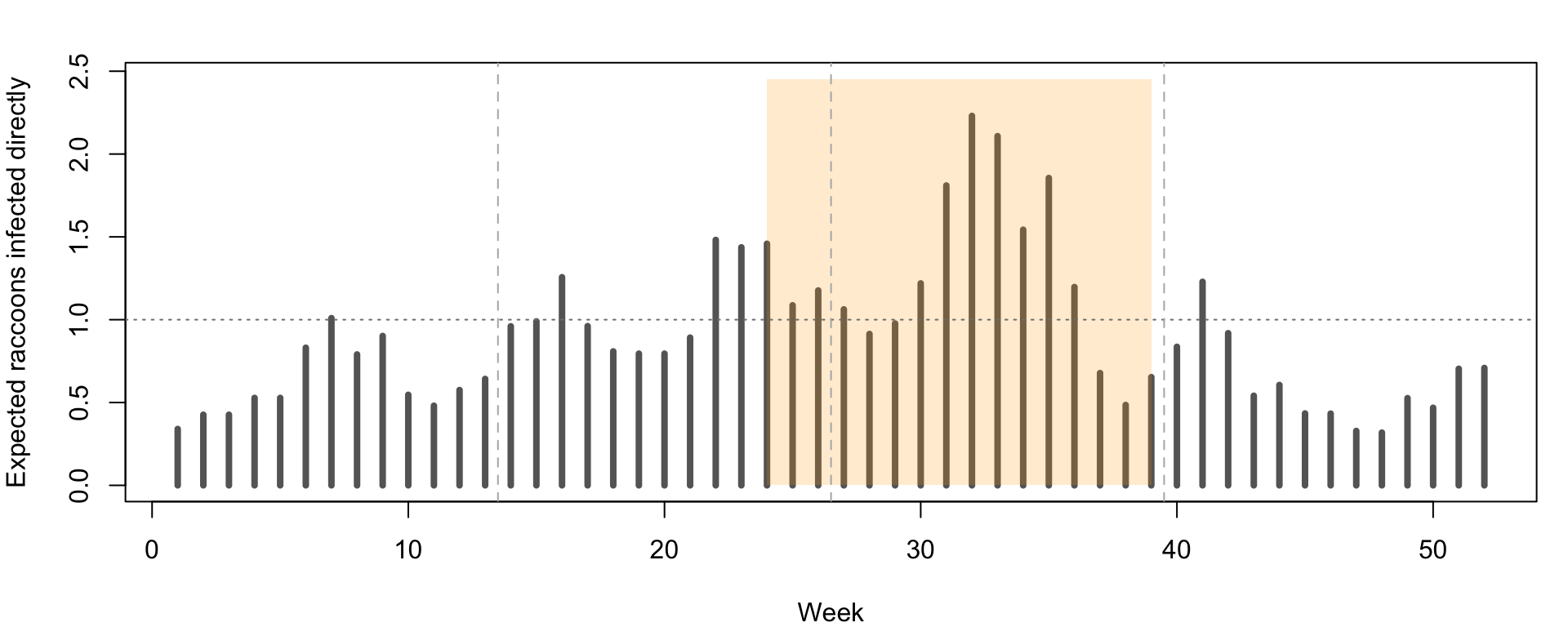
The expected direct infections run from 0.3 to 2.2: highest in the weeks around the middle of the breeding season, and low at its end and from late spring into early summer. This number is not a reproduction number: the raccoons an introduction infects become infectious about six weeks later, in a different week’s network, so the size of an outbreak depends on the weeks that follow as well as the week of introduction. The simulations follow that, and the chance of any onward transmission is a check on them.
Simulations
One netsim() call per level of baseline immunity, each with 5100 simulations; each simulation draws its own introduction week. The outcome is the number of additional cases: raccoons exposed, infectious, or dead by week 104, minus the introduced animal. It counts the whole chain, not only the raccoons the introduced animal infected itself.
sims <- lapply(vax.covs, function(v) {
  p <- param
  p$vax.cov <- v
  netsim(obs, p, init, control)
})
names(sims) <- vax.covs
outcomes <- function(sim) {
df <- as.data.frame(sim)
last <- df[df$time == nsteps, ]
out <- data.frame(week = last$intro.week,
size = last$e.num + last$i.num + last$d.num - 1,
others = last$num - last$r.num - 1)
out$season <- season.of(out$week)
out$attack <- out$size / out$others
out
}
res <- lapply(sims, outcomes)
ci_mean <- function(x) {
m <- mean(x)
se <- sd(x) / sqrt(length(x))
sprintf("%.2f (%.2f, %.2f)", m, m - 1.96 * se, m + 1.96 * se)
}
ci_prop <- function(x) {
p <- mean(x)
se <- sqrt(p * (1 - p) / length(x))
sprintf("%.2f (%.2f, %.2f)", p, max(0, p - 1.96 * se), min(1, p + 1.96 * se))
}
summarize_runs <- function(d) {
data.frame(Simulations = nrow(d),
`P(any additional case)` = ci_prop(d$size >= 1),
`Mean additional cases` = ci_mean(d$size),
`Mean if any` = round(mean(d$size[d$size >= 1]), 2),
`P(5 or more)` = ci_prop(d$size >= 5),
check.names = FALSE)
}Results
Time of year
r0 <- res[["0"]]
tab_season <- do.call(rbind, lapply(split(r0, r0$season, drop = TRUE), summarize_runs))
tab_season <- cbind(Season = rownames(tab_season), tab_season)
season.stats <- sapply(split(r0$size, r0$season), function(x) {
  c(p.any = mean(x >= 1), mean = mean(x), p.five = mean(x >= 5))
})
knitr::kable(tab_season, row.names = FALSE,
caption = "Additional cases per introduction by season of introduction, no vaccination, with 95% intervals over simulations.")| Season | Simulations | P(any additional case) | Mean additional cases | Mean if any | P(5 or more) |
|---|---|---|---|---|---|
| summer (Jul-Sep) | 1206 | 0.44 (0.41, 0.46) | 1.84 (1.66, 2.02) | 4.23 | 0.16 (0.14, 0.18) |
| autumn (Oct-Dec) | 1307 | 0.59 (0.56, 0.62) | 2.62 (2.45, 2.80) | 4.46 | 0.26 (0.23, 0.28) |
| winter (Jan-Mar) | 1294 | 0.64 (0.61, 0.66) | 2.26 (2.12, 2.40) | 3.55 | 0.18 (0.16, 0.21) |
| spring (Apr-Jun) | 1293 | 0.39 (0.36, 0.41) | 0.86 (0.78, 0.94) | 2.22 | 0.04 (0.03, 0.05) |
by.week <- data.frame(
  week = intro.weeks,
  p.any = sapply(intro.weeks, function(w) mean(r0$size[r0$week == w] >= 1)),
  mean = sapply(intro.weeks, function(w) mean(r0$size[r0$week == w])),
  se = sapply(intro.weeks, function(w) sd(r0$size[r0$week == w]) / sqrt(sum(r0$week == w)))
)par(mfrow = c(2, 1), mar = c(4, 4, 1, 1))
plot(intro.weeks, by.week$p.any, pch = 16, col = "#2c3e50", ylim = c(0, 1),
xlim = c(1, 52), xlab = "Week of introduction", ylab = "P(any additional case)")
lines(intro.weeks, potential[intro.weeks, "any"], col = "#e74c3c", lwd = 2)
abline(v = c(13.5, 26.5, 39.5), lty = 2, col = "gray70")
legend("topleft", c("simulated", "expected from the data"), pch = c(16, NA),
lty = c(NA, 1), lwd = c(NA, 2), col = c("#2c3e50", "#e74c3c"), bty = "n")
plot(intro.weeks, by.week$mean, pch = 16, col = "#2c3e50", xlim = c(1, 52),
ylim = c(0, max(by.week$mean + 1.96 * by.week$se, na.rm = TRUE)),
xlab = "Week of introduction", ylab = "Mean additional cases")
ok <- which(by.week$se > 0)
arrows(intro.weeks[ok], by.week$mean[ok] - 1.96 * by.week$se[ok], intro.weeks[ok],
by.week$mean[ok] + 1.96 * by.week$se[ok], angle = 90, code = 3, length = 0.02,
col = "gray50")
segments(c(1, 14, 27, 40), season.stats["mean", ], c(13, 26, 39, 52),
season.stats["mean", ], col = "#e74c3c", lwd = 3)
abline(v = c(13.5, 26.5, 39.5), lty = 2, col = "gray70")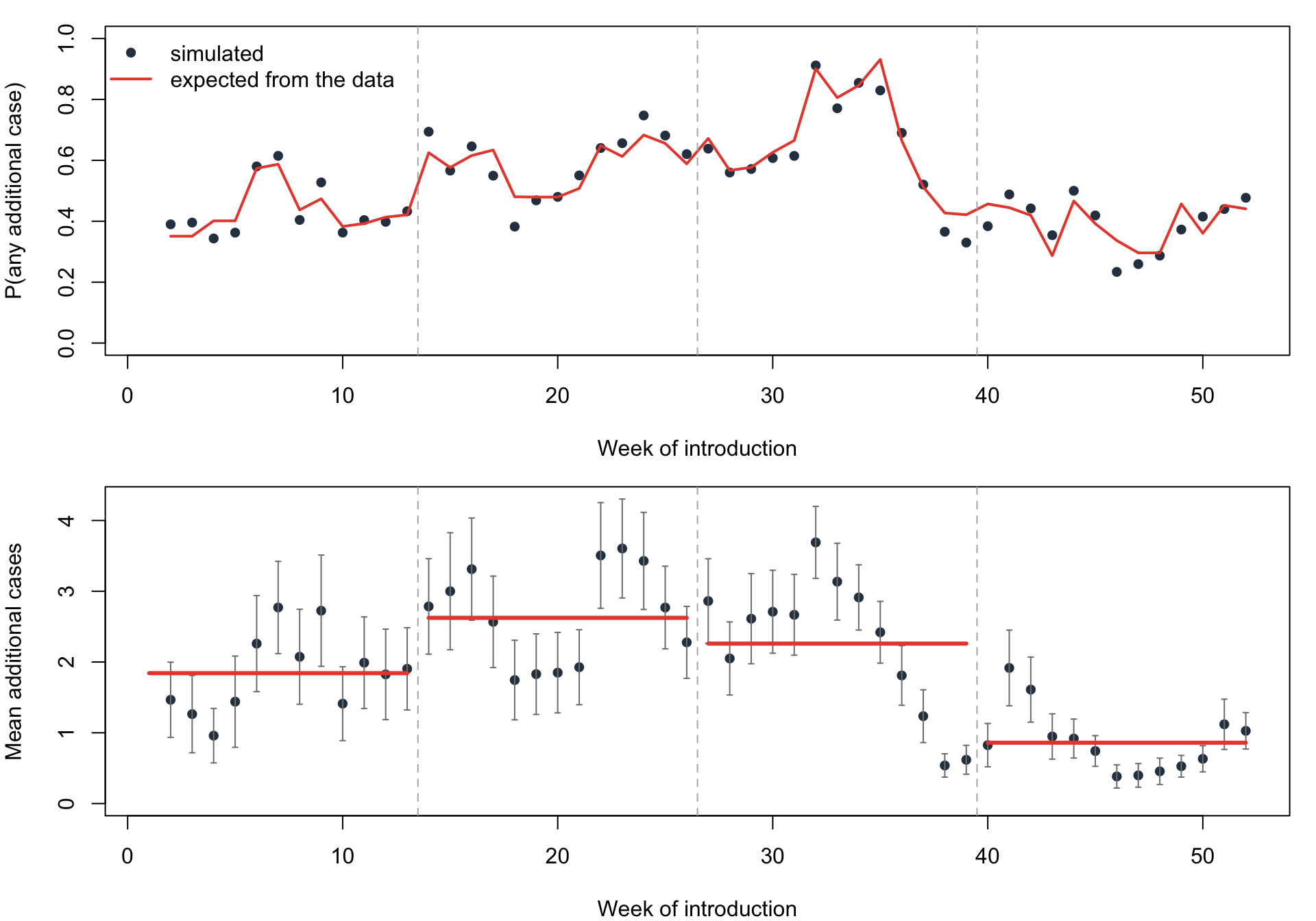
The simulated chance of any additional case follows the expectation computed from the data week by week (correlation 0.95), which checks that the census layer, the contact hours, and the transmission step fit together.
Introductions in winter and autumn most often spread (0.64 and 0.59 of simulations with any additional case), and those in spring least often (0.39). Spring introductions also produce the smallest outbreaks: 0.9 additional cases on average against 1.8 to 2.6 in the other seasons, and five or more in 4% of simulations against 16% to 26%. Autumn introductions produce the largest outbreaks on average, because their chains have the winter weeks of long contacts ahead of them; a winter introduction transmits most often in its own week, but its chains run into the drop in contact time at the end of the breeding season and into spring. Single weeks within a season differ a great deal, so a comparison of single introduction weeks says more about those weeks than about the seasons.
The source paper found that the magnitude and speed of outbreaks depend strongly on the time of year rabies is introduced (Reynolds et al. 2015), and Hirsch et al. (2016) found with the same population that the main driver of that seasonality is contact duration, raised in winter by co-denning, rather than birth pulses or changes in network structure. In this model the season enters only through contact duration among the recorded adults. The spring birth pulse and the autumn dispersal of juveniles, which other analyses tie to rabies seasonality (Elmore et al. 2017), are not in the data.
cols <- c("#3498db", "#e74c3c", "#f39c12", "#27ae60")
df0 <- as.data.frame(sims[["0"]])
curves <- tapply(df0$d.num, list(df0$time, season.of(df0$intro.week)), mean)
par(mfrow = c(1, 1), mar = c(4, 4, 2, 1))
matplot(as.numeric(rownames(curves)), curves, type = "l", lty = 1, lwd = 2, col = cols,
        xlab = "Week", ylab = "Cumulative rabies deaths")
abline(v = 52, lty = 3, col = "gray50")
legend("topleft", legend = paste("introduced in", colnames(curves)), col = cols,
       lwd = 2, bty = "n")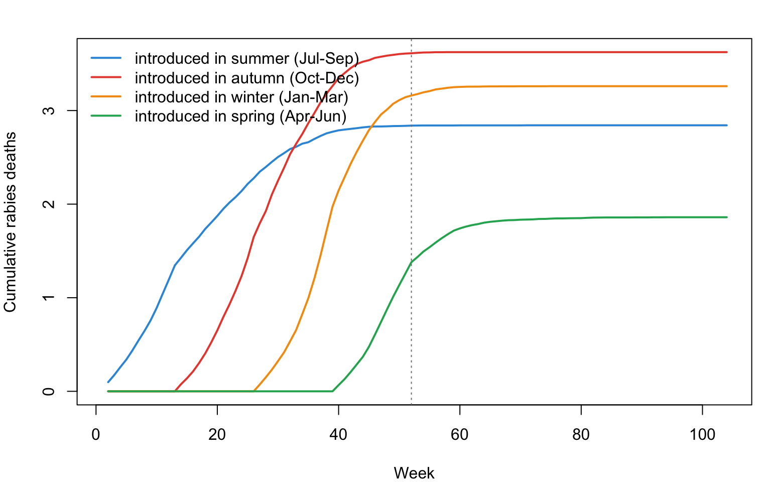
What the transmission assumption implies
The transmission matrix carries the contact hours of every pair that transmitted.
tm <- do.call(rbind, Filter(function(x) NROW(x) > 0, sims[["0"]]$stats$transmat))
q <- round(quantile(tm$hours, c(0.1, 0.25, 0.5, 0.75, 0.9)), 2)
knitr::kable(data.frame(Quantile = names(q), `Contact hours` = q,
                        check.names = FALSE, row.names = NULL),
caption = "Contact hours in the week of transmission, over all transmitting pairs in the unvaccinated simulations.")| Quantile | Contact hours |
|---|---|
| 10% | 0.32 |
| 25% | 1.63 |
| 50% | 9.74 |
| 75% | 35.43 |
| 90% | 89.66 |
Under a constant hazard per hour, long contacts carry most transmission by construction: 80% of transmissions crossed pairs with at least one hour of contact that week, although such pairs are 17% of the pair-weeks in the data, and the median transmitting pair spent 9.7 hours together that week. This is a consequence of the assumption, not a finding about rabies; a model in which a single bite during a brief encounter is enough would give more weight to the many short contacts. Most chains also run their course within year one: 2% of transmissions happen in the replayed year.
Baseline immunity
tab_vax <- do.call(rbind, lapply(names(res), function(v) {
  d <- res[[v]]
  k <- round(as.numeric(v) * n)
  cbind(`Raccoons immune` = sprintf("%d of %d (%.0f%%)", k, n, 100 * k / n),
        summarize_runs(d)[, -1],
        `Attack rate, unvaccinated others` = ci_mean(d$attack))
}))
vax.stats <- sapply(res, function(d) {
  c(p.any = mean(d$size >= 1), mean = mean(d$size), p.five = mean(d$size >= 5),
    attack = mean(d$attack))
})
knitr::kable(tab_vax, row.names = FALSE,
caption = "Additional cases per introduction by the share of raccoons immune at baseline, with the introduction week drawn over the year, and the attack rate among the unvaccinated raccoons other than the introduced one (95% intervals over simulations).")| Raccoons immune | P(any additional case) | Mean additional cases | Mean if any | P(5 or more) | Attack rate, unvaccinated others |
|---|---|---|---|---|---|
| 0 of 24 (0%) | 0.51 (0.50, 0.53) | 1.90 (1.82, 1.98) | 3.70 | 0.16 (0.15, 0.17) | 0.08 (0.08, 0.09) |
| 6 of 24 (25%) | 0.43 (0.41, 0.44) | 1.14 (1.09, 1.19) | 2.66 | 0.08 (0.07, 0.08) | 0.07 (0.06, 0.07) |
| 12 of 24 (50%) | 0.32 (0.31, 0.33) | 0.57 (0.54, 0.60) | 1.79 | 0.01 (0.01, 0.01) | 0.05 (0.05, 0.05) |
| 18 of 24 (75%) | 0.16 (0.15, 0.17) | 0.20 (0.19, 0.22) | 1.27 | 0.00 (0.00, 0.00) | 0.04 (0.04, 0.04) |
p5 <- sapply(res, function(d) tapply(d$size >= 5, d$season, mean))
par(mfrow = c(1, 1), mar = c(4, 4, 2, 1))
matplot(round(as.numeric(colnames(p5)) * n) / n, t(p5), type = "b", pch = 16, lty = 1,
        lwd = 2, col = cols, xlab = "Share of raccoons immune at baseline",
        ylab = "P(5 or more additional cases)", ylim = c(0, max(p5, na.rm = TRUE) * 1.1))
legend("topright", legend = paste("introduced in", rownames(p5)), col = cols,
       pch = 16, lty = 1, bty = "n")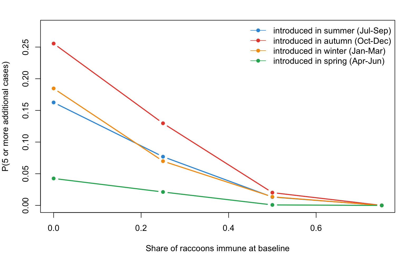
With the introduction week drawn over the year, the mean number of additional cases falls from 1.90 with no immunity to 1.14, 0.57, and 0.20 with 6, 12, and 18 of the 24 raccoons immune, and the chance of five or more additional cases falls from 0.16 to 0.01 with half immune. The attack rate among the unvaccinated raccoons other than the introduced one falls too, from 8% to 4%, so immunity also protects the unvaccinated; part of the fall in additional cases is arithmetic, since with 18 raccoons immune at most five others can be infected.
These numbers are not comparable with published vaccination thresholds. Reynolds et al. (2015), simulating rabies on networks built from these collar data, found that vaccination did not provide an effective barrier until about 85% of raccoons were immune, as summarized by Elmore et al. (2017), and an individual-based landscape model put the seroprevalence needed to prevent epizootics above 60% (Rees et al. 2013). Here a closed group of 24 adults, of whom 16 on average have a recorded contact in a given week, caps any outbreak, and the model has no births, no immigration, and no juveniles, which keep susceptible animals entering a real population. Smaller outbreaks here at a given share immune say that a small, incompletely recorded group stops chains quickly, not that the threshold for a real population is lower.
Sensitivity: the Transmission Hazard
inf.hazard has no direct empirical anchor. The sensitivity runs repeat the unvaccinated simulations at three other hazards, with a quarter of the simulations each.
hazards <- c(0.25, 1, 2)
control_sens <- control
control_sens$nsims <- max(length(intro.weeks), control$nsims / 4)
sens <- lapply(hazards, function(h) {
  p <- param
  p$inf.hazard <- h
  d <- outcomes(netsim(obs, p, init, control_sens))
  c(tapply(d$size, d$season, mean), `P(any), all weeks` = mean(d$size >= 1))
})
tab_sens <- rbind(do.call(rbind, sens),
                  c(tapply(r0$size, r0$season, mean), mean(r0$size >= 1)))
tab_sens <- cbind(inf.hazard = c(hazards, param$inf.hazard), tab_sens)
tab_sens <- tab_sens[order(tab_sens[, "inf.hazard"]), ]knitr::kable(round(tab_sens, 2),
caption = "Mean additional cases by season of introduction, and the share of simulations with any additional case over all weeks, by transmission hazard per contact hour, no vaccination.")| inf.hazard | summer (Jul-Sep) | autumn (Oct-Dec) | winter (Jan-Mar) | spring (Apr-Jun) | P(any), all weeks |
|---|---|---|---|---|---|
| 0.25 | 1.19 | 2.08 | 1.78 | 0.60 | 0.47 |
| 0.50 | 1.84 | 2.62 | 2.26 | 0.86 | 0.51 |
| 1.00 | 2.71 | 3.53 | 3.00 | 1.33 | 0.58 |
| 2.00 | 5.22 | 5.33 | 3.82 | 2.29 | 0.69 |
A higher hazard produces larger outbreaks after introductions in every season, and spring introductions produce the smallest outbreaks at every hazard. The order of the other three seasons depends on the hazard: at 2 per hour, when a three-minute contact transmits about one time in ten, summer introductions do as well as autumn ones, because the many brief summer contacts start to count. Conclusions about which season is riskiest therefore rest on the assumed link between contact time and transmission; the low risk of spring introductions does not.
ImportantWhat the model leaves out
- Kits and juveniles. Kits are too small to collar, so the spring birth pulse, mother-offspring contact, and the autumn dispersal of juveniles are absent, and the population never gains susceptible animals.
- Uncollared raccoons. The collared adults lived in a 20-ha core of a 1,499-ha preserve at 40 to 70 raccoons per km²; contacts with animals outside the core, or with residents that were never collared, are not in the data.
- Collar gaps. A raccoon whose collar was not working is treated as having no contacts, which most likely understates transmission, most of all in winter.
- Bites. Proximity time stands in for bites, and rabid raccoons keep their healthy contact pattern; furious and dumb rabies would change both.
- Vaccination timing. Immunity is fixed at the start of July. ORV baits in the eastern United States are distributed in late summer to early fall, when young raccoons are moving and maternal antibodies have waned (Elmore et al. 2017).
Next Steps
- Behavioral change in rabid raccoons. Furious rabies raises aggression and dumb rabies impairs movement; the source paper tested both. Multiply the contact hours of infectious animals by a stage-specific factor in the infection module and compare.
- Vaccination timing. Replace the baseline immunity with a vaccination module that immunizes in a given week, and interact its timing with the week of introduction.
- Collar gaps. Carry a pair’s contact hours across the weeks in which one of them has no recorded contact but was recorded before and after, and compare the winter results.
- A minimum contact time. Replace the constant hazard with a threshold, so that only pairs with at least 15 or 30 minutes of contact in a week can transmit, closer to the view that brief encounters are not enough for rabies.
- A second layer. The collared raccoons are a fraction of the local population. Add a
netestlayer of contacts with uncollared animals and give the infection module a transmission probability for each layer. The RSV example combines a fixed layer with an estimated one in this way. - Other observed networks. The Animal Social Network Repository holds about 790 networks from more than 45 species (Sah et al. 2019), including twelve proximity networks of Tasmanian devils, the host of devil facial tumor disease. The same
netcensus()workflow applies to any of them. - Fit an ERGM instead. Take one week’s contact network, fit a
netestmodel, and compare epidemics on the fit with epidemics on the observed week; the deposit has no sex or age attributes, so the terms are limited to structure. This is the comparison issue #63 asks for.
References
Data and source studies
- Reynolds JJH, Hirsch BT, Gehrt SD, Craft ME. Raccoon contact networks predict seasonal susceptibility to rabies outbreaks and limitations of vaccination. Journal of Animal Ecology. 2015;84(6):1720-1731. https://doi.org/10.1111/1365-2656.12422. Data: Dryad, https://doi.org/10.5061/dryad.gr40r.
- Sah P, Méndez JD, Bansal S. A multi-species repository of social networks. Scientific Data. 2019;6:44. https://doi.org/10.1038/s41597-019-0056-z. The Animal Social Network Repository copy of the raccoon matrices is the source of
raccoon_contacts.csv. - Hirsch BT, Prange S, Hauver SA, Gehrt SD. Raccoon social networks and the potential for disease transmission. PLoS ONE. 2013;8(10):e75830. https://doi.org/10.1371/journal.pone.0075830.
- Hirsch BT, Reynolds JJH, Gehrt SD, Craft ME. Which mechanisms drive seasonal rabies outbreaks in raccoons? A test using dynamic social network models. Journal of Applied Ecology. 2016;53(3):804-813. https://doi.org/10.1111/1365-2664.12628.
Raccoon rabies and its control
- Elmore SA, Chipman RB, Slate D, Huyvaert KP, VerCauteren KC, Gilbert AT. Management and modeling approaches for controlling raccoon rabies: The road to elimination. PLoS Neglected Tropical Diseases. 2017;11(3):e0005249. https://doi.org/10.1371/journal.pntd.0005249.
- Rees EE, Pond BA, Tinline RR, Bélanger D. Modelling the effect of landscape heterogeneity on the efficacy of vaccination for wildlife infectious disease control. Journal of Applied Ecology. 2013;50(4):881-891. https://doi.org/10.1111/1365-2664.12101.
- Tinline R, Rosatte R, MacInnes C. Estimating the incubation period of raccoon rabies: a time-space clustering approach. Preventive Veterinary Medicine. 2002;56(1):89-103. https://doi.org/10.1016/s0167-5877(02)00126-5.
Animal social networks and epidemic simulation
- Farine DR, Whitehead H. Constructing, conducting and interpreting animal social network analysis. Journal of Animal Ecology. 2015;84(5):1144-1163. https://doi.org/10.1111/1365-2656.12418.
- Webber QMR, Brigham RM, Park AD, Gillam EH, O’Shea TJ, Willis CKR. Social network characteristics and predicted pathogen transmission in summer colonies of female big brown bats (Eptesicus fuscus). Behavioral Ecology and Sociobiology. 2016;70(5):701-712. https://doi.org/10.1007/s00265-016-2093-3.
The rabies parameters here are illustrative choices within published ranges, selected to show the mechanics of an observed-network model. They are not calibrated to surveillance data, and the 24 collared adults are a fraction of the population they lived in.