library(EpiModel)7 New DCMs
This tutorial documents how to use EpiModel to solve new deterministic compartmental models (DCMs). New model types incorporate model compartments, parameters, and structures different from the built-in SI/SIR/SIS model types in EpiModel. This extension tutorial assumes a solid familiarity with both R programming and epidemic model parameterization the other tutorials. If you are not familiar with DCMs or running this model class in EpiModel, consult the Basic DCMs with EpiModel in Chapter 3 tutorial.
7.1 The EpiModel DCM Framework
First load the EpiModel package:
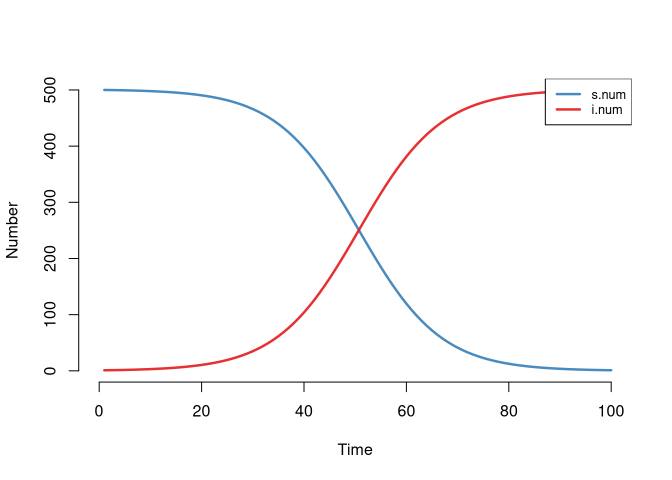
To start let’s examine the mathematical syntax for our basic SI model in a closed population (no births or deaths). We first run this model in EpiModel to see the normal syntax that avoids any specific reference to the model function specifying the mathematical structure. As detailed in the basic tutorial, EpiModel automatically chooses the correct model function as a result of the input parameters, initial conditions, and control settings.
param <- param.dcm(inf.prob = 0.5, act.rate = 0.25)
init <- init.dcm(s.num = 500, i.num = 1)
control <- control.dcm(type = "SI", nsteps = 100)
mod <- dcm(param, init, control)
plot(mod)
7.1.1 Model Functions
Within EpiModel, DCMs are solved using the deSolve package, using this framework to define a model as a function that includes calculations for dynamic rates and the system of differential equations for each compartment in the model. To see what one of these looks like, we can use the control.dcm argument print.mod = TRUE. When the dcm function is run with this, only the model structure is printed to the console.
control <- control.dcm(type = "SI", nsteps = 100, print.mod = TRUE)
mod <- dcm(param, init, control)
function (t, t0, parms)
{
with(as.list(c(t0, parms)), {
num <- s.num + i.num
lambda <- inf.prob * act.rate * i.num/num
if (!is.null(parms$inter.eff) && t >= inter.start) {
lambda <- lambda * (1 - inter.eff)
}
si.flow <- lambda * s.num
dS <- -si.flow
dI <- si.flow
list(c(dS, dI, si.flow), num = num)
})
}
<bytecode: 0x560bdedf6d90>
<environment: namespace:EpiModel>The standard specification for model functions is with the top two lines to wrap the input and output into a list structure. The mathematical calculation of main derivatives, dS and dI, are an arithmetic function of the force of infection, lambda and the size of the susceptible population, s.num. The base model functions include a modifier on the lambda to simulate an intervention if those parameters are specified in the model.
An alternative method for accessing the built-in model functions is to consult the internal help page for those functions.
?dcm.modsThere are currently a total of 12 model types: three disease types (SI, SIR, and SIS), two group number specifications (one versus two groups), and two demographic settings (open versus closed populations). An equivalent method to access the same model function as above is by printing the internal model function.
print(mod_SI_1g_cl)function (t, t0, parms)
{
with(as.list(c(t0, parms)), {
num <- s.num + i.num
lambda <- inf.prob * act.rate * i.num/num
if (!is.null(parms$inter.eff) && t >= inter.start) {
lambda <- lambda * (1 - inter.eff)
}
si.flow <- lambda * s.num
dS <- -si.flow
dI <- si.flow
list(c(dS, dI, si.flow), num = num)
})
}
<bytecode: 0x560bdedf6d90>
<environment: namespace:EpiModel>7.1.2 Steps to Writing a Model Function
Each mathematical model solved using EpiModel must have its own R function. The core function structure should be the the same for each model:
- It must include the overall function structure, including the two lines at the top and two lines at the bottom. These lines should not be changed at all. They pass in the initial conditions and fixed parameters to be evaluated over time.
- Next input are all dynamic calculations, including varying parameters like
lambda(the force of infection), which changes as a function of infected population size. Here, we include the calculation fornum, the total population size. This is not dynamic in this particular model because of the closed population, but it allows for a shorthand formula forlambda. The values fors.numandi.num, the number susceptible and infected, are passed into this function via the initial conditions we set ininit.dcm. Dynamic calculations also include composite statistics that you would like to output with the model (e.g.,prevalence <- i.num/num). - The differential equations should next be specified very similarly to how they are written in Stella or Madonna software. The names of the differential equations are arbitrary (e.g.,
dSbelow) but must be consistent with the output list. The derivatives for the model not only include the compartment sizes for the disease states, but also any flows in the model (si.flowin this model); that is because the flow sizes are calculated using the same method of numerical integration as the compartment sizes. - The output list is what deSolve outputs in solving the model. This list should include, at the least, all the differential equations that you have defined in the function, including the flows. This list first specifies the differential equation in a combined vector:
c(dS, dI, si.flow). Always list the derivative objects first, in this combined vector format, and in the same order that they are entered in the initial conditions list. After writing these equations, one can also output dynamic statistics from the model. These should be named in the manner below to ensure that the output object has appropriate column names. - Finally, the function should be named something unique and relevant, and then saved to memory. We will show the details of that below.
7.1.3 Parameters, Initial Conditions, and Controls
To define the parameters, initial state sizes, and control settings for the model specifications use the the param.dcm, init.dcm, and control.dcm helper functions.
- Parameters are entered in the same manner they are with built-in models, but there must be consistency between the parameter names entered in
param.dcmand the variables called within your new model function. - The initial conditions are also entered similarly, but it is vital to remember that states must be in exacty the same order as the differential equations in the function output. If you are experiencing unexpected model results, this is the first thing to check. Also, remember to enter all flow sizes as both initial conditions here. The variable names for flows show end in
.flow: this tells EpiModel to calculate the flow sizes at each time step as a lagged difference rather than a cumulative size. If the flows are not named to end with.flow, errors will be the result. - Finally controls are also entered similarly, but one no longer uses the
typeparameter, and instead uses thenew.modparameter to specify the model function.
Details of these steps will be further described in the two examples below.
7.2 Example 1: SEIR Model
EpiModel includes a built-in SIR model, but here we show how to model an SEIR disease like Ebola. The E compartment in this disease is an exposed state in which the person is not infectious to others. Following some basic parameters for Ebola in the popular science to date, we model this disease using parameters for \(R_0\), the average durations spent in the exposed and infected phases, and the case fatality rate. This model will use a simplifying assumption that the only deaths in the population are due to Ebola.
Persons infected then either die from infection or recovery at an equal rate, defined by the average time spent in the infected state. Other simplifying assumptions here are that dead persons do not transmit disease (many infections have occurred this way) and that the rate of contacts remains the same over the infected phase (it probably declines, but there is not good data on this).
7.2.1 Model Function
We use four parameters in the model: R0 is the initial reproductive number, e.dur is the duration of the exposed state, i.dur is the duration of the infectious state, and cfr is the case fatality rate expressed as a proportion of those who will die among those infected. Given estimates on \(R_0\) and the duration of infection, we infer a simplistic lambda by mathematical rearrangement.
The four differential equations are defined as a function of state sizes and parameters. For the infected state, in-flows are from the exposed stage and out-flows are either to the recovered state (1 - the CFR will recover) or death (CFR will die).
SEIR <- function(t, t0, parms) {
  with(as.list(c(t0, parms)), {

    # Population size
    num <- s.num + e.num + i.num + r.num

    # Effective contact rate and FOI from a rearrangement of Beta * c * D
    ce <- R0 / i.dur
    lambda <- ce * i.num/num

    dS <- -lambda*s.num
    dE <- lambda*s.num - (1/e.dur)*e.num
    dI <- (1/e.dur)*e.num - (1 - cfr)*(1/i.dur)*i.num - cfr*(1/i.dur)*i.num
    dR <- (1 - cfr)*(1/i.dur)*i.num

    # Compartments and flows are part of the derivative vector
    # Other calculations to be output are outside the vector, but within the containing list
    list(c(dS, dE, dI, dR,
           se.flow = lambda * s.num,
           ei.flow = (1/e.dur) * e.num,
           ir.flow = (1 - cfr)*(1/i.dur) * i.num,
           d.flow = cfr*(1/i.dur)*i.num),
         num = num,
         i.prev = i.num / num,
         ei.prev = (e.num + i.num)/num)
  })
}
In the model output, we include the four derivatives, but also several other calculated time-series to analyze later. These are all included as named elements of the list, with compartments and flows specified as derivatives in the named vector and other summary statistics included in the output list.
7.2.2 Model Parameters
For model parameters, we specify the following values. Our sensitivity analysis will vary the CFR, given the potential for variability of this across health systems. The starting population is roughly 1 million persons in which 10 have been exposed at the outset. Note that we specify the initial value for all the flows named in the model, with a starting value of 0 (i.e., there are no transitions at the outset of the model simulation). We simulate this model over 500 days, specifying that our model function is SEIR as defined above.
param <- param.dcm(R0 = 1.9, e.dur = 10, i.dur = 14, cfr = c(0.5, 0.7, 0.9))
init <- init.dcm(s.num = 1e6, e.num = 10, i.num = 0, r.num = 0,
                 se.flow = 0, ei.flow = 0, ir.flow = 0, d.flow = 0)
control <- control.dcm(nsteps = 500, dt = 1, new.mod = SEIR)
mod <- dcm(param, init, control)
The model shows that three models were run, where the CFR was varied. All the output in the model matches our model function specs.
modEpiModel Simulation
=======================
Model class: dcm
Simulation Summary
-----------------------
No. runs: 3
No. time steps: 500
Model Parameters
-----------------------
R0 = 1.9
e.dur = 10
i.dur = 14
cfr = 0.5 0.7 0.9
Model Output
-----------------------
Variables: s.num e.num i.num r.num se.flow ei.flow ir.flow
d.flow num i.prev ei.prev7.2.3 Model Results
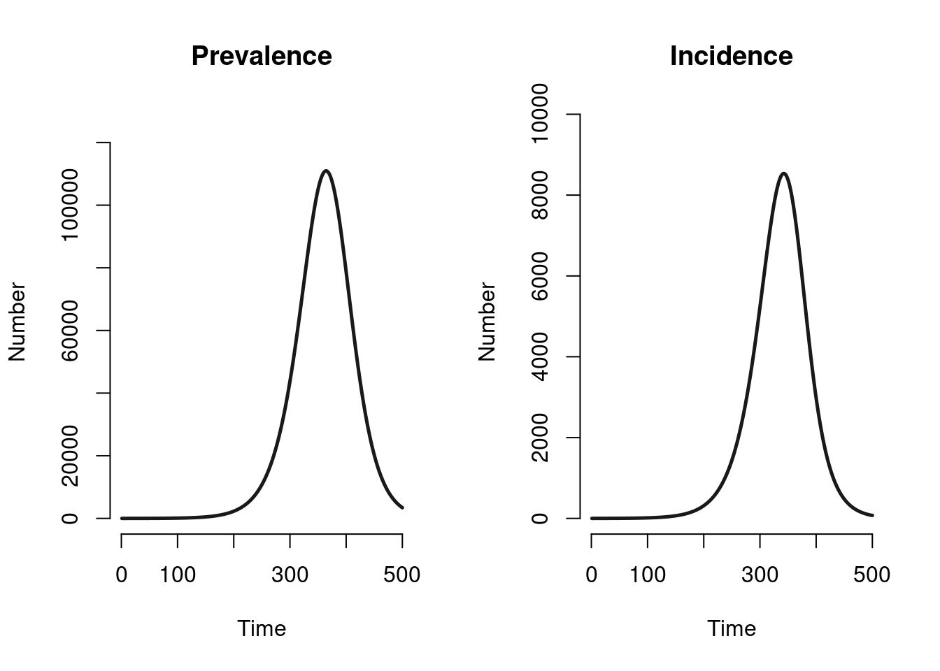
Let’s first ignore the sensitivity analysis and examine the model with the middle CFR of 70%. Here is what the prevalence and incidence are from the model. In the initial epidemic, the prevalence curve is approximated by an exponential growth model. The peak incidence occurs roughly one year into the epidemic.
par(mfrow = c(1, 2))
plot(mod, y = "i.num", run = 2, main = "Prevalence")
plot(mod, y = "se.flow", run = 2, main = "Incidence")
Now, let’s examine what impact the CFR has on prevalence, both in raw numbers and as proportions. The higher CFR actually results in a higher prevalence, in both absolute and proportional terms. Why is that the case? Look to the definition of the force of infection in our model. The higher CFR has the effect of reducing the population size, but the effective contact rate is fixed. Therefore, in a circular way, a higher prevalence epidemic results in a higher probability of contacting an infected person leading to higher prevalence, and so on.
par(mfrow = c(1, 2))
plot(mod, y = "i.num", main = "Number Infected")
plot(mod, y = "i.prev", main = "Percent Infected", ylim = c(0, 0.5), legend = "full")
Many assumptions of the model may be reworked, a quarantine or vaccine intervention introduced, or more complex contact patterns (e.g., contact with the dead) included. This has just demonstrated with a relatively parsimonious model how to include novel specifications for model structure and parameterizations.
7.3 Example 2: Variable Mixing Model
The second example model is a reproduction of the variable mixing model in which the “Q statistic” is used to vary the propensity for mixing between high and low activity groups (in terms of their sexual partner change rates). For a sensitivity analysis in the model, we vary the Q statistic from fully dissortative mixing (high-risk people only mix with low-risk people) to partially dissortative mixing to proportional (random) mixing to partially assortative mixing to fully assortative mixing (high-risk people only mix with high-risk people). Our model is based on a DCM programmed in Madonna that is featured in “An Introduction to Infectious Disease Modeling” by Vynnycky and White.
7.3.1 Model Function
This model function is specified similiarly to the examples above. Many more calculations are needed for the flexibility in mixing. This is an SIS model in a closed population, so the equations for each group are balanced (the in-flow for the infected state is the outflow of the susceptible state). Also note that we calculated the total disease prevalence and have included it as model output. Finally, as before, the order of the differential equation formulas and their corresponding output objects matches.
Qmod <- function(t, t0, parms) {
  with(as.list(c(t0, parms)), {

    ## Dynamic Calculations ##

    # Population size and prevalence
    h.num <- sh.num + ih.num
    l.num <- sl.num + il.num
    num <- h.num + l.num
    prev <- (ih.num + il.num) / num

    # Contact rates for high specified as a function of
    #   mean and low rates
    c.high <- (c.mean*num - c.low*l.num) / h.num

    # Mixing matrix calculations based on variable Q statistic
    g.hh <- ((c.high*h.num) + (Q*c.low*l.num)) /
            ((c.high*h.num) + (c.low*l.num))
    g.lh <- 1 - g.hh
    g.hl <- (1 - g.hh) * ((c.high*h.num) / (c.low*l.num))
    g.ll <- 1 - g.hl

    # Probability that contact is infected based on mixing probabilities
    p.high <- (g.hh*ih.num/h.num) + (g.lh*il.num/l.num)
    p.low <- (g.ll*il.num/l.num) + (g.hl*ih.num/h.num)

    # Force of infection for high and low groups
    lambda.high <- rho * c.high * p.high
    lambda.low <- rho * c.low * p.low


    ## Derivatives ##
    dS.high <- -lambda.high*sh.num + nu*ih.num
    dI.high <- lambda.high*sh.num - nu*ih.num

    dS.low <- -lambda.low*sl.num + nu*il.num
    dI.low <- lambda.low*sl.num - nu*il.num


    ## Output ##
    list(c(dS.high, dI.high, dS.low, dI.low),
         num = num, prev = prev)
  })
}
7.3.2 Model Parameters
Parameters for this model use completely different names than the built-in epidemic parameters. We specify the mean contact rate in c.mean, the contact rate for the low group in c.low, the probability of infection per contact in rho, and the rate of recovery in nu. Finally, the Q parameter controls how the high and low groups mix, from purely dissortative mixing when Q = -0.45, to proportional mixing when Q = 0, to purely assortative mixing when Q = 1.
param <- param.dcm(c.mean = 2, c.low = 1.4, rho = 0.75, nu = 6,
                   Q = c(-0.45, -0.33, 0, 0.5, 1))
Following the example in the textbook, this epidemic is simulated in a very large population in which a small proportion (2%) are in the high-activity group. We are not monitoring any flows in our model, so we do not include them in the initial conditions as we did in Example 1.
init <- init.dcm(sh.num = 2e7*0.02, ih.num = 1,
                 sl.num = 2e7*0.98, il.num = 1)
The rates are in the parameters are specified in terms of yearly time units, so the model may be solved over 25 years in increments of (roughly) weeks by specifying the nsteps and dt parameters below. The new.mod parameter must specify the new model function.
control <- control.dcm(nsteps = 25, dt = 0.02, new.mod = Qmod)7.3.3 Model Simulations
Running the model uses the same syntax as before.
mod <- dcm(param, init, control)Printing the model object shows the parameters and available output. Note that now that we have used both parameter and compartment names that differ from the built-in model types, one should not expect to see any of those in the output.
modEpiModel Simulation
=======================
Model class: dcm
Simulation Summary
-----------------------
No. runs: 5
No. time steps: 25
Model Parameters
-----------------------
c.mean = 2
c.low = 1.4
rho = 0.75
nu = 6
Q = -0.45 -0.33 0 0.5 1
Model Output
-----------------------
Variables: sh.num ih.num sl.num il.num num prevSimilar to the built-in model types, the as.data.frame method works with any dcm model objects to put all the output from one model run in a useful data.frame format. The default prints model run 1.
head(as.data.frame(mod)) run time sh.num ih.num sl.num il.num num prev
1 1 1.00 400000.0 1.0000000 19600000 1.000000 2e+07 9.999999e-08
2 1 1.02 400000.1 0.8996819 19600000 1.317867 2e+07 1.108774e-07
3 1 1.04 400000.2 0.8130011 19599999 1.561663 2e+07 1.187332e-07
4 1 1.06 400000.3 0.7378402 19599999 1.744571 2e+07 1.241205e-07
5 1 1.08 400000.3 0.6724247 19599999 1.877556 2e+07 1.274990e-07
6 1 1.10 400000.4 0.6152670 19599999 1.969734 2e+07 1.292501e-07head(as.data.frame(mod, run = 5)) run time sh.num ih.num sl.num il.num num prev
1 5 1.00 400000.0 1.000000 19600000 1.0000000 2e+07 9.999999e-08
2 5 1.02 399999.6 1.420437 19600000 0.9057428 2e+07 1.163090e-07
3 5 1.04 399999.0 2.017639 19600000 0.8203700 2e+07 1.419004e-07
4 5 1.06 399998.1 2.865924 19600000 0.7430442 2e+07 1.804484e-07
5 5 1.08 399996.9 4.070853 19600000 0.6730069 2e+07 2.371930e-07
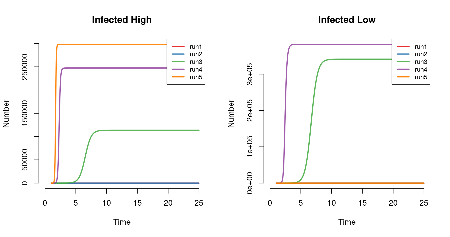
6 5 1.10 399995.2 5.782364 19600000 0.6095712 2e+07 3.195967e-07The plots below show the number infected in the high and low groups across model runs. Prevalence is highest in the high group with purely assortative mixing (run = 5), but lowest in the low group under this condition. This highlights an important aspect of assortative mixing, with the infection “trapped” in the high-group under this extreme condition.
par(mfrow = c(1, 2))
plot(mod, y = "ih.num", legend = "full", main = "Infected High")
plot(mod, y = "il.num", legend = "full", main = "Infected Low")
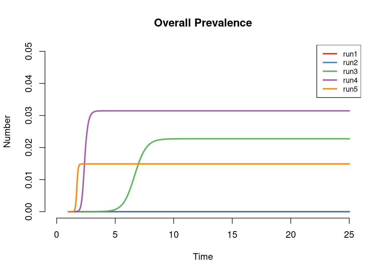
This next plot shows overall disease prevalence in both groups. The prevalence was saved in the model function in the prev output, so here we plot that outcome. This shows the full impact of variable mixing on the epidemic: under both levels of dissortative mixing (runs 1 and 2) the epidemic goes extinct. The highest prevalence is observed with moderate assortivity (run 4). Even under proportional mixing (run 3), the prevalence at equilibrium is higher than with purely assortivity (run 5), but epidemic does not reach that prevalence until several years later. In the purely assortative model, the overall prevalence is essentially limited by the size of the high-risk group.
par(mfrow = c(1,1))
plot(mod, y = "prev", ylim = c(0, 0.05), legend = "full", main = "Overall Prevalence")