param <- param.dcm(inf.prob = 0.2, act.rate = 0.25)
init <- init.dcm(s.num = 500, i.num = 1)
control <- control.dcm(type = "SI", nsteps = 500)3 Basic DCMs
3.1 Introduction
This tutorial provides a mathematical and theoretical background for deterministic, compartmental models (DCMs), with instructions on how to run the built-in models designed for learning in EpiModel. For information on how to extend these models to simulate novel epidemiological processes, see the related tutorial New DCMs with EpiModel in Chapter 7.
Deterministic compartmental models solve differential equations representing analytic epidemic systems in continuous time. The models are deterministic because their solutions are fixed mathematical functions of the input parameters and initial conditions, with no stochastic variability in the disease and demographic transition processes. The models are compartmental because they divide the population into groups representing discrete disease states (e.g., susceptible and infected), and further on demographic, biological, and behavioral traits that influence disease transmission. In contrast to the stochastic models presented below, individuals within the population are not discretely represented.
3.2 A Basic SI Model
Starting with a basic Susceptible-Infected (SI) disease model in which there is random mixing within the population, the size of each compartment over time is represented by the equations:
\[ \begin{align} \frac{dS}{dt} &= -\lambda S \notag \\[4pt] \frac{dI}{dt} &= \lambda S \end{align} \]
where \(\lambda\) is the force of infection and represents \(\frac{\beta c I}{N}\). \(\beta\) is the probability of transmission per contact, \(c\) is the rate of contact per person per unit time, \(I\) is the number infected at time \(t\) and and \(N\) is the population size at time \(t\) (we drop the \(t\) subscript as it is implicit throughout).
Because ``contact’’ has been defined several ways in the modeling literature, we use the word act to represent the action, such as face-to-face discussion or sexual intercourse, by which disease may be transmitted. The force of infection is multiplied by the current state sizes of the \(S\) to solve the differential equation yielding the rate of change for the compartment.
To simulate a deterministic model in EpiModel, use the dcm function. Prior to running the model, it is necessary to parameterize it. Model parameters, initial conditions, and controls settings are input into three helper functions that organize the model framework. In param.dcm, the epidemic model parameters are entered. The inf.prob argument sets the transmission probability per act, and act.rate sets the acts per person per unit time. The init.dcm function collects the initial conditions for the model, and since this is an SI model it is necessary to specify the initial number susceptible and infected at \(t_1\). The control.dcm finally collects other structural model controls like the model type and number of time steps for the simulation.
The model parameters, initial conditions, and controls are then entered as inputs into the dcm function to run the model and save the output in our object mod.
mod <- dcm(param, init, control)Options for analyzing the results are consistent across all the model classes and types. Printing the model object provides basic information on model input and output, including model parameters and data variables for plotting and analysis.
modEpiModel Simulation
=======================
Model class: dcm
Simulation Summary
-----------------------
Model type: SI
No. runs: 1
No. time steps: 500
No. groups: 1
Model Parameters
-----------------------
inf.prob = 0.2
act.rate = 0.25
Model Output
-----------------------
Variables: s.num i.num si.flow numThe output shows that two compartments and one flow are available. In EpiModel, regardless of the model class, compartments are discrete disease states and flows are the transitions between states; when demographic processes are introduced, flows represent transitions in and out of the population. The i.num compartment is the size of the infected population at each of the solved time steps. The endogenous disease flow names represent the starting and ending state: si.flow is the number of people moving from \(S\) to \(I\) at each time step. In epidemiological terms, i.num and si.flow are disease prevalence and incidence.
To plot the results of the model we use the generic plot function, which by default plots all the model compartment state sizes over time.
plot(mod)
After examining the plot, one can investigate the the size of each compartment at a specific time step. That is available with the summary function. At \(t_{150}\), 22.5% of the population have become infected, and disease incidence is 4.37 new infections.
summary(mod, at = 150)EpiModel Summary
=======================
Model class: dcm
Simulation Summary
-----------------------
Model type: SI
No. runs: 1
No. time steps:
No. groups: 1
Model Statistics
------------------------------
Time: 150 Run: 1
------------------------------
n pct
Suscept. 112.845 0.225
Infect. 388.155 0.775
Total 501.000 1.000
S -> I 4.311 NA
------------------------------ 3.3 SIR Model with Demography
In a Susceptible-Infectious-Recovered (SIR) model, infected individuals transition from disease into a life-long recovered state in which they are never again susceptible. Here we model an SIR disease by adding to our basic SI model a recovery process. We also introduce demographic processes so that persons enter and exit the population through births and deaths. The model is represented by the following system of differential equations:
\[ \begin{align} \frac{dS}{dt} &= -\lambda S + bN - \mu_s S \notag \\[4pt] \frac{dI}{dt} &= \lambda S - \nu I - \mu_i I \notag \\[4pt] \frac{dR}{dt} &= \nu I - \mu_r R \end{align} \]
where \(b\) is the birth rate, \(\mu\) are the mortality rates specific for each compartment, and \(\nu\) is the recovery rate; note that across EpiModel, birth and mortality rates are more generally referred to as arrival and departure rates, respectively. In an SIR model, the recovery rate is the reciprocal of the average duration of disease; likewise, the reciprocal of the death rates are the average life expectancy for persons in those compartments.
3.3.1 Simulation
In EpiModel, introducing new transition processes into the model is straightforward. In param.dcm, parameters for the recovery rate, birth rate, and state-specific death rates are entered. These parameters imply that the birth rate is slightly higher than the underlying death rate among susceptibles, and that there is disease-induced mortality because the di.rate is larger than the other two death rates. In init.dcm, it is necessary to specify the number of initially recovered, even if that is 0. In control.dcm, the dt argument may be used to obtain model results in fractional time units (i.e., results are available for \(t_1\), \(t_{1.5}\), \(\dots\), \(t_{499.5}\), \(t_{500}\)).
param <- param.dcm(inf.prob = 0.2, act.rate = 1, rec.rate = 1/20,
                   a.rate = 1/95, ds.rate = 1/100, di.rate = 1/80, dr.rate = 1/100)
init <- init.dcm(s.num = 1000, i.num = 1, r.num = 0)
control <- control.dcm(type = "SIR", nsteps = 500, dt = 0.5)
mod <- dcm(param, init, control)
3.3.2 Plotting
Next we plot the results of the model to demonstrate several plot arguments. First, the par function is used to change some default graphical options. In the left plot, the popfrac=FALSE argument plots the compartment size (rather than prevalence) and alpha increases the transparency of the lines for better visualization. By default, the plot function will plot the prevalences for all compartments in the model, but in the right plot we override that using the y argument to specify that disease incidence (the si.flow element of the model object) should be plotted.
par(mar = c(3.2, 3, 2, 1), mgp = c(2, 1, 0), mfrow = c(1, 2))
plot(mod, popfrac = FALSE, alpha = 0.5,
     lwd = 4, main = "Compartment Sizes")
plot(mod, y = "si.flow", lwd = 4, col = "firebrick",
     main = "Disease Incidence", legend = "n")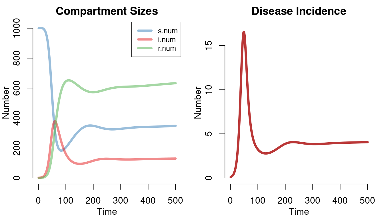
It is possible to specify a single line color, a vector of colors, or a color palette using the col argument, and the legend options are set using the legend argument.
3.3.3 Summaries
Previously, the time-specific model values were calculated with the summary function. To visualize that information, use the comp_plot function. This plot provides a state-flow diagram that is often presented in the epidemiological literature. The plot shows the three state sizes and flows at \(t_{50}\).
par(mfrow = c(1, 1))
comp_plot(mod, at = 50, digits = 1)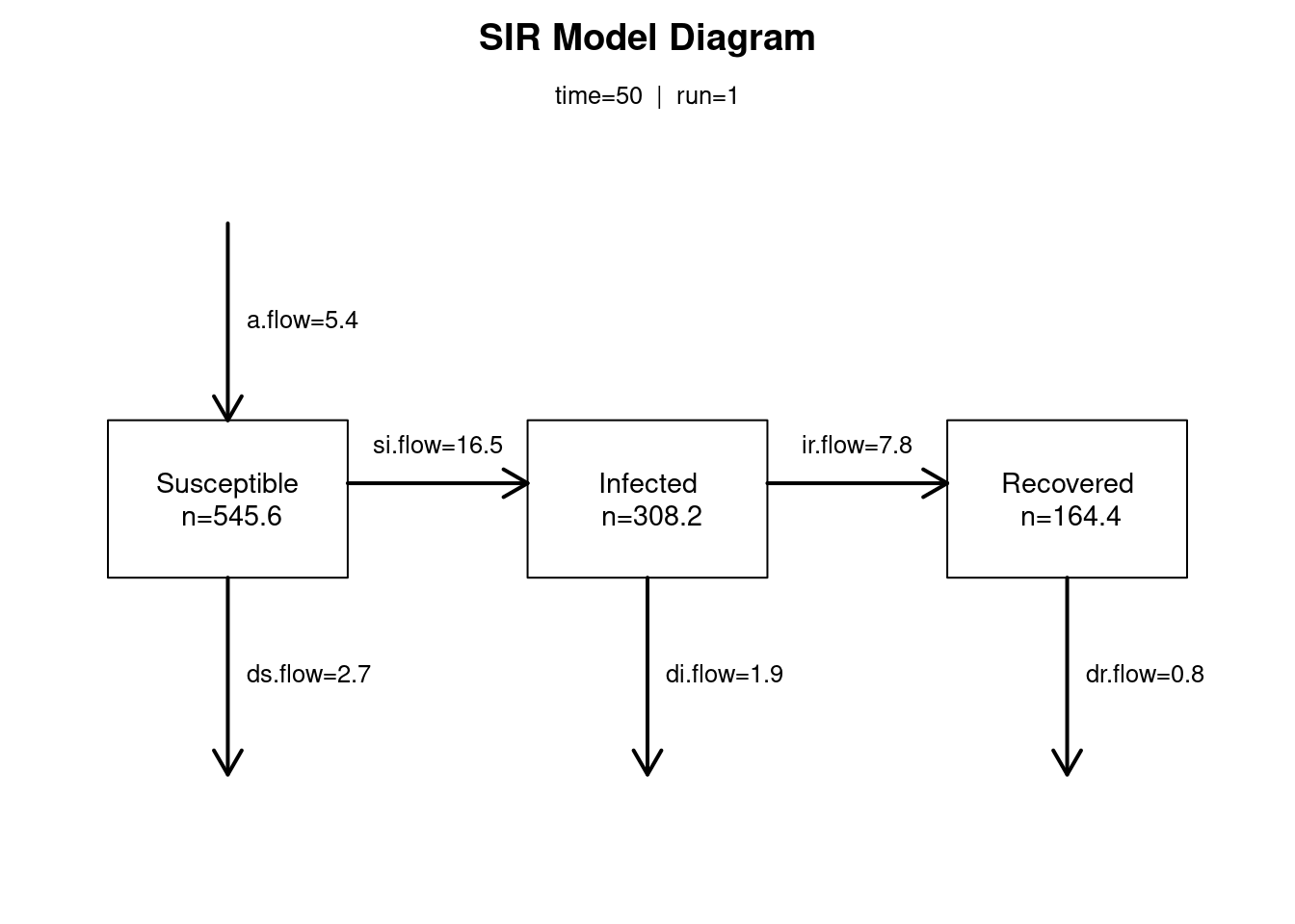
3.4 SIS Model with Sensitivity Analyses
Often of scientific interest with mathematical models is to investigate how epidemics vary under different parameter values. A key design feature of dcm class models in EpiModel is facilitating these sensitivity analyses. This section illustrates a Susceptible-Infected-Susceptible (SIS) disease, an example of which is a bacterial sexually transmitted infection like gonorrhea. For ease of presentation, we model this in a closed population, but those processes may be added in the same way as our SIR model above.
The SIS model is represented by the following system of differential equations: \[ \begin{align} \frac{dS}{dt} &= -\lambda S + \nu I \notag \\[4pt] \frac{dI}{dt} &= \lambda S - \nu I \end{align} \] where the \(\nu\) parameter now represents “recovery” back into the susceptible state (no one achieves life-long immunity from disease). The force of infection and recovery equations mirror each other, since individuals flow back and forth between states.
In EpiModel, running an SIS model requires specifying type="SIS" and supplying a rec.rate parameter, just as with the SIR model. To run a sensitivity analysis, the parameter to be varied is entered as a vector of values rather than a single value. Here, we vary the act.rate parameter from 0.25 to 0.50 acts acts per person per unit time in increments of 0.05 acts. The dcm function will therefore run 6 models with different act.rate parameters, holding all others constant.
param <- param.dcm(inf.prob = 0.2, act.rate = seq(0.25, 0.5, 0.05), rec.rate = 0.02)
init <- init.dcm(s.num = 500, i.num = 1)
control <- control.dcm(type = "SIS", nsteps = 350)
mod <- dcm(param, init, control)
When printing model output, it is clear that a sensitivity model has been run because the output indicates 6 runs, with the appropriate range of values for the act.rate parameter.
modEpiModel Simulation
=======================
Model class: dcm
Simulation Summary
-----------------------
Model type: SIS
No. runs: 6
No. time steps: 350
No. groups: 1
Model Parameters
-----------------------
inf.prob = 0.2
act.rate = 0.25 0.3 0.35 0.4 0.45 0.5
rec.rate = 0.02
Model Output
-----------------------
Variables: s.num i.num si.flow is.flow num3.4.1 Extracting Output
The output of each compartment or flow is a data frame with columns for each model run and rows for each time step. To extract all the model output for all compartments and flows from a specific run, we can use as.data.frame. Below we extract model output from the fifth model run for the first six time steps. The run-specific data frame may also be saved out to its own object for further analysis.
head(as.data.frame(mod, run = 5)) run time s.num i.num si.flow is.flow num
1 5 1 500.0000 1.000000 0.09302333 0.02071469 501
2 5 2 499.9277 1.072309 0.09973410 0.02221239 501
3 5 3 499.8502 1.149830 0.10692634 0.02381805 501
4 5 4 499.7671 1.232939 0.11463421 0.02553939 501
5 5 5 499.6780 1.322033 0.12289420 0.02738470 501
6 5 6 499.5825 1.417543 0.13174535 0.02936283 5013.4.2 Plotting
When plotting a sensitivity analysis, EpiModel uses color to differentiate the model runs. Below is a two-panel plot of disease prevalence and incidence across all 6 models. By default, plotting a sensitivity model will show the disease prevalence: the proportion of persons infected in each model run at each time step.
par(mfrow = c(1,2), mar = c(3.2,3,2.5,1))
plot(mod, alpha = 1, main = "Disease Prevalence")
plot(mod, y = "si.flow", col = "Greens", alpha = 0.8, main = "Disease Incidence")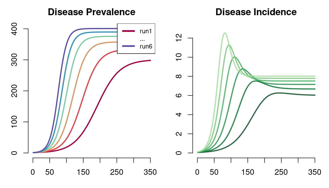
EpiModel uses a robust color palette system to set the default colors for the model-specific results. The underlying functionality is based on the RColorBrewer package, which provides access to visually distinct color palettes. The default color palette is featured for the prevalence plot, but any palette in display.brewer.all() may be set using the col argument, as with the incidence plot.
The color argument also accepts vectors of colors as well. For example, the following are also acceptable color specifications for a sensitivity analysis plot. It is also possible to set run-specific line types in a similar fashion using the lty argument.
plot(mod, col = "black")
plot(mod, col = 1:6)
plot(mod, col = c("black", "red", "blue", "green", "purple", "pink"))
plot(mod, col = rainbow(3), lty = rep(1:2, each = 3), legend = "full")
3.4.3 Varying Multiple Parameters
One may vary multiple parameters simultaneously, with the limitation that the number of model runs implied must be equal across varying parameters. For example, if one specifies act.rate as a vector of length six, and one is also interested in simultaneously varying the transmission probability, the length of that inf.prob vector must also be six. Below is an example showing those two parameters simultaneously varied. In total, six models are simulated in this sensitivity analysis. There are three different act rates, and for each act rate, there are two different transmission probabilities to model. The varying act and transmission parameters will then be evaluated in that order, with the first model having act.rate=0.2 and inf.prob=0.1, and the last model having act.rate=0.6 and inf.prob=0.2.
act.rates <- c(0.2, 0.2, 0.4, 0.4, 0.6, 0.6)
inf.probs <- c(0.1, 0.2, 0.1, 0.2, 0.1, 0.2)
param <- param.dcm(inf.prob = inf.probs, act.rate = act.rates,
                   rec.rate = 0.02)
mod <- dcm(param, init, control)
plot(mod)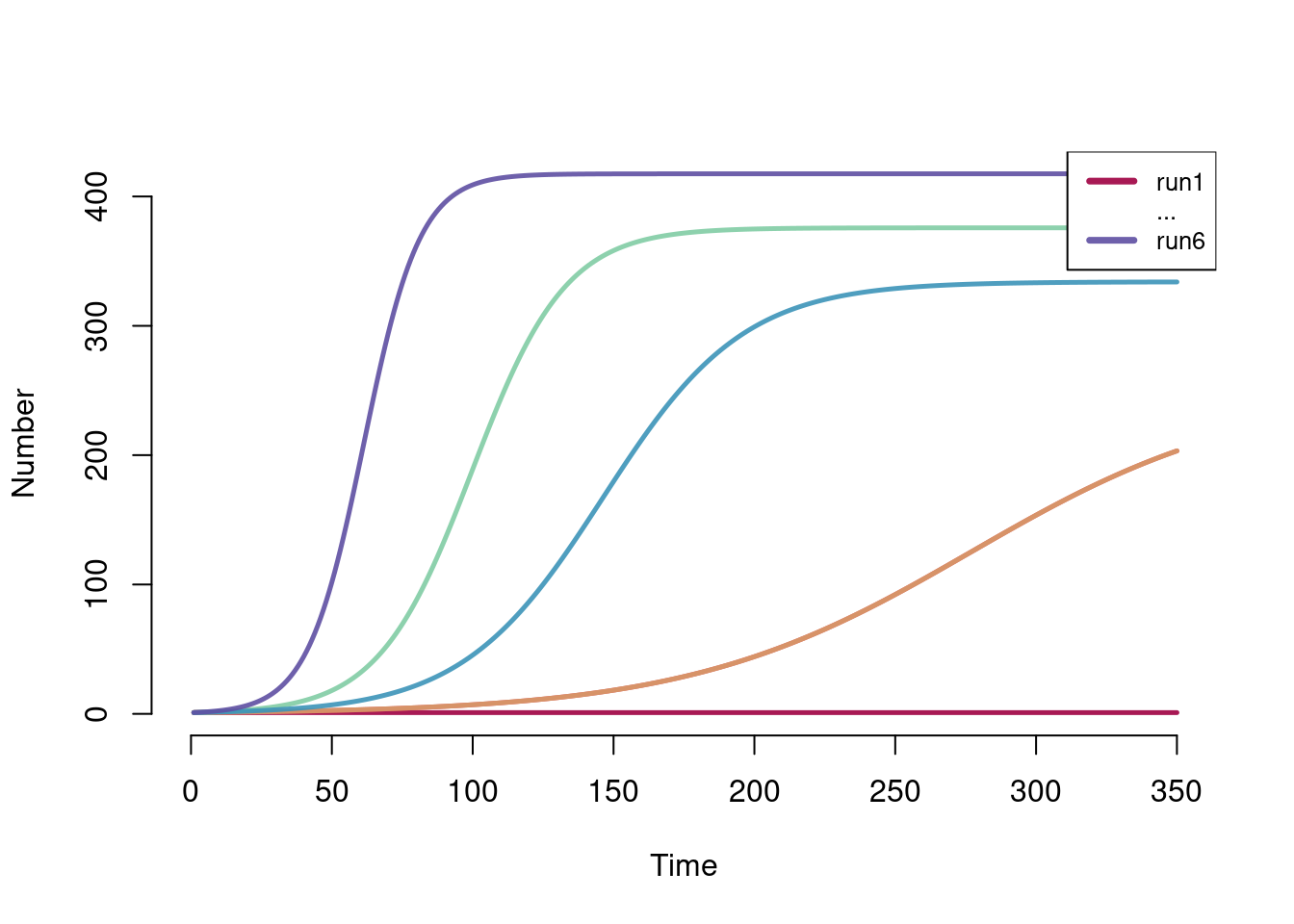
3.4.4 SI Model with Demography
EpiModel also includes heterogeneous two-group models, which break the random mixing patterns implied by one-group models. These two-group models are available for all three model classes, but for network models they are called two-mode (or bipartite models) in accordance with network science terminology. In the two-group models as they are currently structured, mixing between groups is purely heterogeneous: one group only has contacts with the other group and there are no within-group contacts. This framework would be appropriate for epidemic modeling over heterosexual partnerships, with the simplifying assumption of no same-sex contacts.
3.4.5 Mathematical Structure
We build upon the basic SI model featured above. The model now includes four compartments, two disease states \(\times\) two groups, requiring the following set of four differential equations. The equation variables are sub-scripted by group number; in dcm we only need to specify the group-specific parameters for the force of infection, birth rate, and death rates.
\[ \begin{align} \frac{dS_{g1}}{dt} &= -\lambda_{g1}S_{g1} + f_{g1}N_{g1} - \mu_{s,g1}S_{g1} \notag \\[4pt] \frac{dI_{g1}}{dt} &= \lambda_{g1}S_{g1} - \mu_{i,g1}I_{g1} \notag \\[4pt] \frac{dS_{g2}}{dt} &= -\lambda_{g2}S_{g2} + f_{g2}N_{g2} - \mu_{s,g2}S_{g2} \notag \\[4pt] \frac{dI_{g2}}{dt} &= \lambda_{g2}S_{g2} - \mu_{i,g2}I_{g2} \end{align} \]
The critical heterogeneous mixing component is embedded within the group-specific \(\lambda\) transmission probabilities. The formula for the two lambdas that specifies mixing is:
\[ \begin{align} \lambda_{g1} &= \tau_{g1} \times \alpha_{g1} \times \frac{I_{g2}}{N_{g2}} \notag \\[4pt] \lambda_{g2} &= \tau_{g2} \times \alpha_{g2} \times \frac{I_{g1}}{N_{g1}} \end{align} \]
In words, the force of infection for Group 1 is the product of the group one transmission probability per act, the Group 1 act rate per unit time, and the probability that an infected is selected among the possible Group 2 contacts. The difference with the one-group model is that group-specific \(\tau\) and \(\alpha\) parameters are allowed. The probability of contact with an infected person is not based on the prevalence of all infected persons, but only those of the opposite group. The group-specific \(\tau\) parameter is the probability of infection to that group member (e.g., \(\tau_{g1}\) is the probability that a member of Group 1 is infected given contact with a member of Group 2).
3.5 Balancing Acts
Another concern for models like this is the act rate parameter, \(\alpha\). In the formulas for the group-specific \(\lambda\) above, it was implied that each group may have its own act rate. However, in practice with these purely heterogeneous mixing models, the act rate of one group has a defined mathematical relationship with the act rate of the other group:
\[ \begin{align} \alpha_{g1}N_{g1} &= \alpha_{g2}N_{g2} \end{align} \]
The number of acts within each group is their act rate times their group size. The total number of acts in one group in this heterogeneous mixing model must equal the total number of acts in the other. To accomplish we use act rate “balancing.” This is particularly important in an open population model since the group population sizes may change over time.
There are a variety of methods for balancing, but the base models in EpiModel use a simple approach. One specifies an \(\alpha\) parameter for either Group 1 or Group 2, and specify which group has the controlling rate. For example, if one specifies \(\alpha_{g1}\), then the act rate for Group 1 is fixed at that value and the rate for Group 2 is derived over time by rearranging the equation above as follows:
\[ \begin{align} \alpha_{g2} &= \frac{\alpha_{g1}N_{g1}}{N_{g2}} \end{align} \]
One may implement more flexible balancing that averages two act rates or deals with changes in other ways, following the methods in the New DCMs with EpiModel tutorial in Chapter 7.
3.5.1 Parameterizing Groups
With the dcm function, it is simple to implement two-group models. One only needs to set the group-specific initial state sizes and model parameters. The names of the parameters for the first group has not changed: the sizes and parameters specific to group one are those without the g2 suffix. An important use of two-group models is to allow for some biological or behavioral heterogeneity between groups that impacts disease transmission. In the model below, we specify that the transmission probability for Group 1 is four times as high as that of Group 2. This could represent a four-fold higher risk of infection for females (Group 1) than for males (Group 2). We enforce the act rate balancing as above, by specifying an act rate for Group 1 only and also using the balance = "g1" argument.
param <- param.dcm(inf.prob = 0.4,  inf.prob.g2 = 0.1, act.rate = 0.25, balance = "g1",
                   a.rate = 1/100, a.rate.g2 = NA, ds.rate = 1/100, ds.rate.g2 = 1/100,
                   di.rate = 1/50, di.rate.g2 = 1/50)
init <- init.dcm(s.num = 500, i.num = 1, s.num.g2 = 500, i.num.g2 = 0)
control <- control.dcm(type = "SI", nsteps = 500)
mod <- dcm(param, init, control)
Note also how the group-specific birth rates are input. Because these heterogeneous mixing models are ideal for heterosexual disease transmission in which groups represent sexes, we can model Group 1 as females and Group 2 as males. In this case, the birth rate into a population is not a function of the total population size but that of the female group. In that case, one specifies a birth rate for females only and sets the Group 2 birth rate to NA. If so this is done, new births are evenly allocated between the two groups based on the size of group one and the rate specified by a.rate.
After simulating the model, we print it to show its contents. The number of compartments and flows available to plot and analyze has now doubled. The Group 1 outcomes are those without the g2 suffix.
modEpiModel Simulation
=======================
Model class: dcm
Simulation Summary
-----------------------
Model type: SI
No. runs: 1
No. time steps: 500
No. groups: 2
Model Parameters
-----------------------
inf.prob = 0.4
act.rate = 0.25
a.rate = 0.01
ds.rate = 0.01
di.rate = 0.02
inf.prob.g2 = 0.1
a.rate.g2 = NA
ds.rate.g2 = 0.01
di.rate.g2 = 0.02
balance = g1
Model Output
-----------------------
Variables: s.num i.num s.num.g2 i.num.g2 si.flow a.flow
ds.flow di.flow si.flow.g2 a.flow.g2 ds.flow.g2 di.flow.g2
num num.g2The default plot shows the prevalence of all four compartments in the model. Two-group models with sensitivity analyses begin to visually overwhelm the plotting. One may freely deviate from the default plotting options to specify other compartments or flows to visualize.
plot(mod)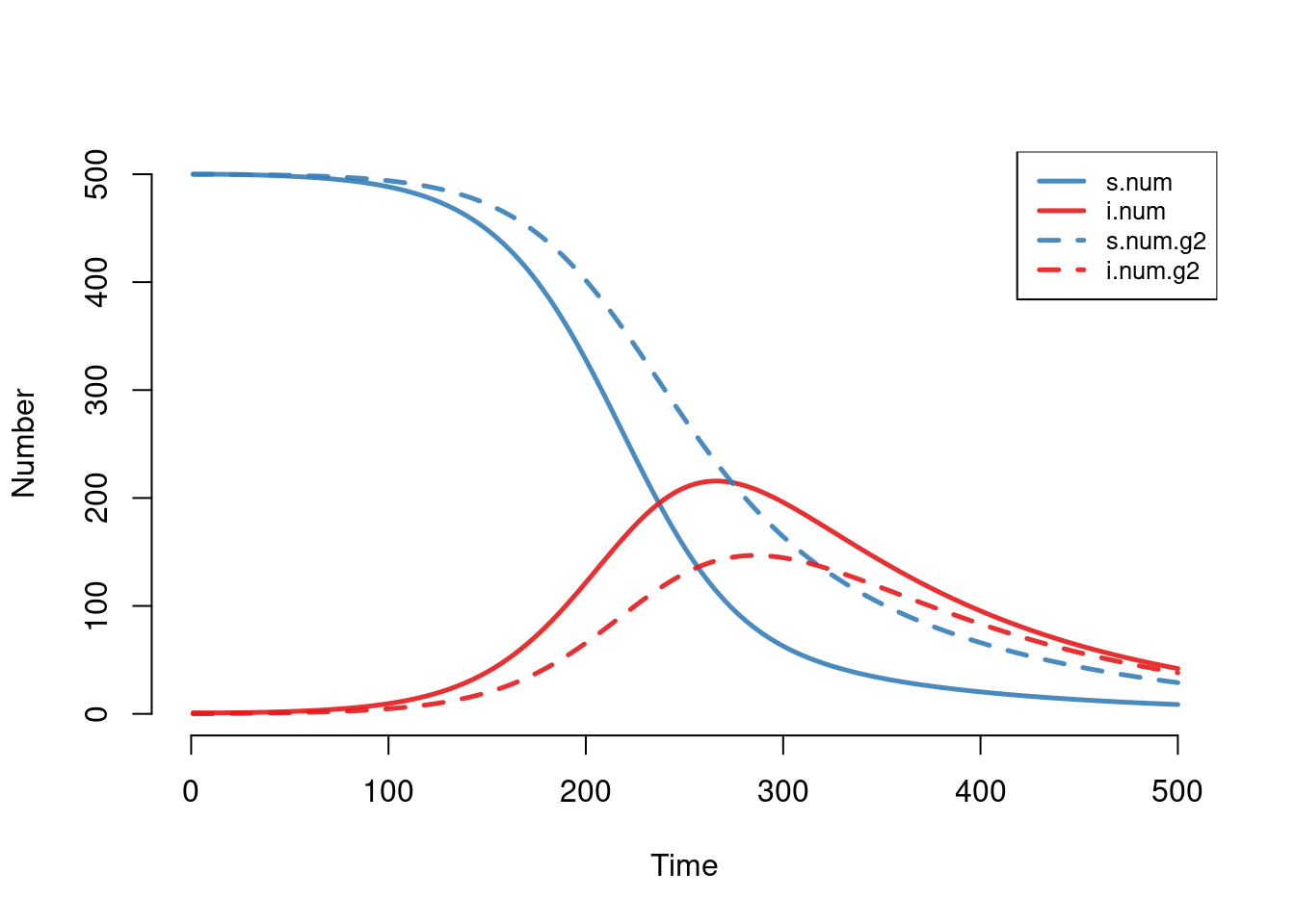
3.6 Next Steps
This tutorial has provided the basics to get started with exploring DCMs with EpiModel. From here, you have a choice where to go next. If you are mainly interested in DCMs and want to learn how to build your own DCMs that eliminate some of the assumptions and specifications of these basic DCMs, the New DCMs with EpiModel tutorial in Chapter 7 is appropriate. If instead you would like to learn about stochastic modeling of epidemics with the same type of built-in models, the Basic ICMs with EpiModel in Chapter 5 will provide a background on Stochastic Individual Contact Models. Knowledge of ICMs serves as a good foundation to running Stochastic Network Models.