param <- param.icm(inf.prob = 0.2, act.rate = 0.25)
init <- init.icm(s.num = 500, i.num = 1)
control <- control.icm(type = "SI", nsims = 10, nsteps = 300)
mod <- icm(param, init, control)5 Basic ICMs
5.1 Introduction
This tutorial provides a mathematical and theoretical background for stochastic individual contact models (ICMs), with instructions on how to simulate the built-in models designed for learning stochastic modeling in EpiModel. If you are new to epidemic modeling, we suggest that you start with our tutorial Basic DCMs with EpiModel in Chapter 3 to get a background in that standard epidemic modeling approach. Some of the material here assumes familiarity with DCMs.
Stochastic ICMs are designed to be agent-based microsimulation analogs to the deterministic compartmental models (DCMs) solved with the dcm function. The main differences between the two model classes are as follows.
- Parameters are random draws: these are stochastic models in which all of the rates and risks governing transitions between states are random draws from distributions summarized by those rates or probabilities, including normal, Poisson, and binomial distributions.
- Time is discrete: ICMs are simulated in discrete time, in contrast to the continuous time of DCMs. In discrete time, everything within a time step happens as a series of processes, since there is no instantaneous occurrence of events independent of others, possible in continuous-time models. This has the potential to introduce some artificiality into the modeling if the unit for the time step is large because transitions that might occur within that time step cannot necessarily be considered independent. In general, caution is needed when simulating any discrete-time model with long unit time steps or large rate parameters, given the potential for competing risks.
- Units are individuals: ICMs simulate disease spread over a simulated population of individually identifiable elements; in contrast, DCMs treat the population as an aggregate whole which is infinitely divisible, with individual elements in this population neither identifiable nor accessible for modeling purposes. The implications of this are relatively minor if the stochastic simulations occur on a sufficiently large population, but there are some critical modeling considerations of individual-based simulations that will be reviewed in the examples below.
A goal of EpiModel is to facilitate comparisons across different model classes, so the interface and functionality of the stochastic models in icm, the main function to run ICMs, is very similar to dcm, the main function to run DCMs. The syntax and argument names for the parameters and initial state sizes are the same.
5.2 SI Model Stochasticity
We introduce ICM class models by using the same model parameterization as the basic DCM SI model the Basic DCMs Tutorial in Chapter 3, with one person infected, an act rate of 0.25 per time step, and an infection probability of 0.2 per act. We simulate this model 10 times over 300 time steps. Note that the parameterization helper functions now end with .icm.
By default, the function prints the model progress. These agent-based simulation models generally take longer to run than DCMs, especially for larger populations and longer time ranges, because transition processes must be simulated for each individual at each time step. The model results may be printed, summarized, and plotted in very similar a fashion to the dcm models.
modEpiModel Simulation
=======================
Model class: icm
Simulation Summary
-----------------------
Model type: SI
No. simulations: 10
No. time steps: 300
No. groups: 1
Model Parameters
-----------------------
inf.prob = 0.2
act.rate = 0.25
Model Output
-----------------------
Variables: s.num i.num num si.flowIn contrast to dcm class objects, the summary function does not take a run argument. The output summarizes the mean and standard deviation of model results at the requested time step across all simulations. Here, we request those summaries at time step 125; the output shows the compartment and flow averages across those 10 simulations.
summary(mod, at = 125)EpiModel Summary
=======================
Model class: icm
Simulation Details
-----------------------
Model type: SI
No. simulations: 10
No. time steps: 300
No. groups: 1
Model Statistics
------------------------------
Time: 125
------------------------------
mean sd pct
Suscept. 274.5 126.674 0.548
Infect. 226.5 126.674 0.452
Total 501.0 0.000 1.000
S -> I 3.6 1.578 NA
------------------------------ Summary statistic values like means and standard deviations may be of interest for analysis and visualization, so the as.data.frame function for icm objects provides this. As described in the function help page (see help("as.data.frame.icm")), the output choices are for the time-specific means, standard deviations, and individual simulation values.
head(as.data.frame(mod, out = "mean")) time s.num i.num num si.flow
1 1 500.0 1.0 501 0.0
2 2 499.9 1.1 501 0.1
3 3 499.7 1.3 501 0.2
4 4 499.6 1.4 501 0.1
5 5 499.5 1.5 501 0.1
6 6 499.5 1.5 501 0.0tail(as.data.frame(mod, out = "vals", sim = 1)) sim time s.num i.num num si.flow
295 1 295 0 501 501 0
296 1 296 0 501 501 0
297 1 297 0 501 501 0
298 1 298 0 501 501 0
299 1 299 0 501 501 0
300 1 300 0 501 501 05.2.1 Plotting
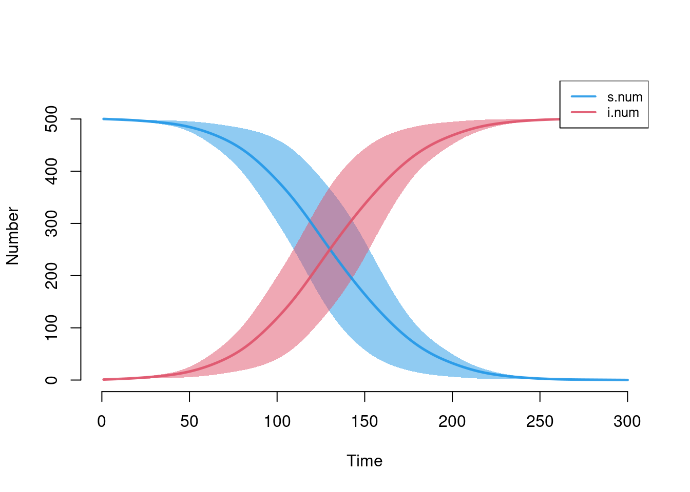
Plotting stochastic model results requires thinking through what summary measures best represent the epidemic. For some models, it may be sufficient to plot the simulation means, but in others visualizing the individual simulations is necessary. The plotting function for icm objects generates these visual outputs simply but robustly. Standard plotting output includes the means across simulations along with the inter-quartile range of values; both are smoothed values by default.
plot(mod)
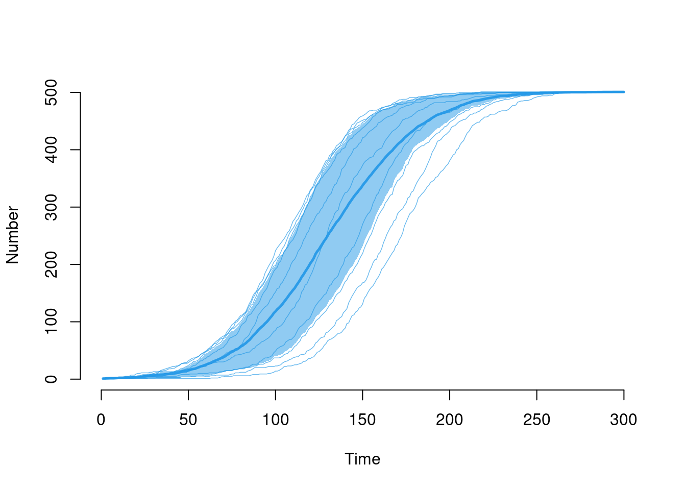
Each of the elements may be toggled on or off using the plotting arguments listed in help("plot.icm"). Here, we add the individual simulation lines to the default plot using sim.lines and remove the smoothing of the means and quantile band.
plot(mod, y = "i.num", sim.lines = TRUE, mean.smooth = FALSE, qnts.smooth = FALSE)
5.3 SIR DCM/ICM Comparison
One question for comparative modeling is how results vary with model structure holding constants the epidemic parameters. EpiModel allows for easy comparison between model classes using the same parameters. Here, we show how to compare a DCM with an ICM of an SIR epidemic in an open population. First, the deterministic model is run with the following parameters.
param <- param.dcm(inf.prob = 0.2, act.rate = 0.8, rec.rate = 1/50,
                   a.rate = 1/100, ds.rate = 1/100, di.rate = 1/90, dr.rate = 1/100)
init <- init.dcm(s.num = 900, i.num = 100, r.num = 0)
control <- control.dcm(type = "SIR", nsteps = 300)
det <- dcm(param, init, control)
Note that 10% of the population are set as infected at \(t_0\); with just one person initially infected, it typically takes discrete-time, individual-based models longer to grow an epidemic. This is a unique property of agent-based models that may better represent reality. Here, the goal is a close approximation by minimizing these differences. The icm model is simulated 10 times, with the same parameters as the deterministic model. In this model, the contact, transmission given contact, recovery, birth, and death processes are all governed by random draws from binomial distributions with parameters set by the rates specified here; recall that across EpiModel, birth and mortality rates are more generally referred to as arrival and departure rates, respectively.
param <- param.icm(inf.prob = 0.2, act.rate = 0.8, rec.rate = 1/50,
                   a.rate = 1/100, ds.rate = 1/100, di.rate = 1/90,
                   dr.rate = 1/100)
init <- init.icm(s.num = 900, i.num = 100, r.num = 0)
control <- control.icm(type = "SIR", nsteps = 300, nsims = 10)
sim <- icm(param, init, control)
For a third model, we change our ICM model to toggle off the stochastic elements of the birth death processes. Instead of setting the number of new births and deaths in each compartment at each time step as random draws from binomial distributions with rate parameters set by the arguments, these transition flows are calculated by rounding the product of the rate and the state size. Note that we can recycle the param and init from the previous model.
control <- control.icm(type = "SIR", nsteps = 300, nsims = 10,
                       a.rand = FALSE, d.rand = FALSE)
sim2 <- icm(param, init, control)
5.3.1 Comparing Means
In our plot, the deterministic results are shown in the solid line, the first stochastic results in the dashed line, and second stochastic results in the dotted line. In this example, the three lines are generally consistent, which is as expected since we are only visualizing the means, we have a sufficiently large population, and the demographic transition rates are relatively low. Note the use of the add argument to place a new set of lines on top of an existing plot window.
plot(det, alpha = 0.75, lwd = 4, main = "DCM and ICM Comparison")
plot(sim, qnts = FALSE, sim.lines = FALSE, add = TRUE, mean.lty = 2, legend = FALSE)
plot(sim2, qnts = FALSE, sim.lines = FALSE, add = TRUE, mean.lty = 3, legend = FALSE)
5.3.2 Comparing Variance
There is no variability in the deterministic model, but the variability between the second and third models is of interest. Here we compare the variability of the death flow among infected in the first fully stochastic model and the second limited stochastic model with deterministic deaths. In the fully stochastic model, there is a relatively wide range of numbers of infected deaths over time, whereas there is little variability in the limited stochastic model.
par(mfrow = c(1,2), mar = c(3,3,2,1), mgp = c(2,1,0))
plot(sim, y = "di.flow", mean.line = FALSE,
     sim.lines = TRUE, sim.alpha = 0.15, ylim = c(0, 20),
     main = "di.flow: Full Stochastic Model")
plot(sim2, y = "di.flow", mean.line = FALSE,
     sim.lines = TRUE, sim.alpha = 0.15, ylim = c(0, 20),
     main = "di.flow: Limited Stochastic Model")
There are still minor variations in the death flows at some time points because the number infected at each time point is still a function of the random transmission processes in the model. For a time-specific analysis of variance, we can compare the standard deviations of the two model results at time step 50 (about when the infected death incidence peaks) using the data extraction through the as.data.frame function.
icm.compare <- rbind(round(as.data.frame(sim, out = "sd")[50,], 2),
                     round(as.data.frame(sim2, out = "sd")[50,], 2))
row.names(icm.compare) <- c("full", "lim")
icm.compare
time s.num i.num num r.num si.flow ir.flow ds.flow di.flow dr.flow
full 50 12.04 15.22 19.01 16.04 2.25 2.86 1.17 1.99 1.79
lim 50 13.51 23.94 19.32 13.30 1.96 2.17 1.14 1.93 1.25
a.flow
full 2.58
lim 3.335.4 SIS Model with Demography
Next we model a two-group Susceptible-Infected-Susceptible (SIS) model in which there are two groups that mix purely heterogeneously. The model is parameterized similar to the deterministic two-group SIR model featured in the Basic DCMs Tutorial in Chapter 3. We use the same act rate balancing considerations. One must also specify group-specific recovery rates. In this model, we simulate a disease in which the first group has twice the probability of infection, but recovers back into the susceptible state at twice the rate as the second group. This might occur, for example, if first group differentially had access to curative treatment for disease.
param <- param.icm(inf.prob = 0.2, inf.prob.g2 = 0.1, act.rate = 0.5, balance = "g1",
                   rec.rate = 1/25, rec.rate.g2 = 1/50, a.rate = 1/100, a.rate.g2 = NA,
                   ds.rate = 1/100, ds.rate.g2 = 1/100, di.rate = 1/90, di.rate.g2 = 1/90)
init <- init.icm(s.num = 500, i.num = 1, s.num.g2 = 500, i.num.g2 = 1)
control <- control.icm(type = "SIS", nsteps = 500, nsims = 10)

set.seed(1)
sim <- icm(param, init, control)
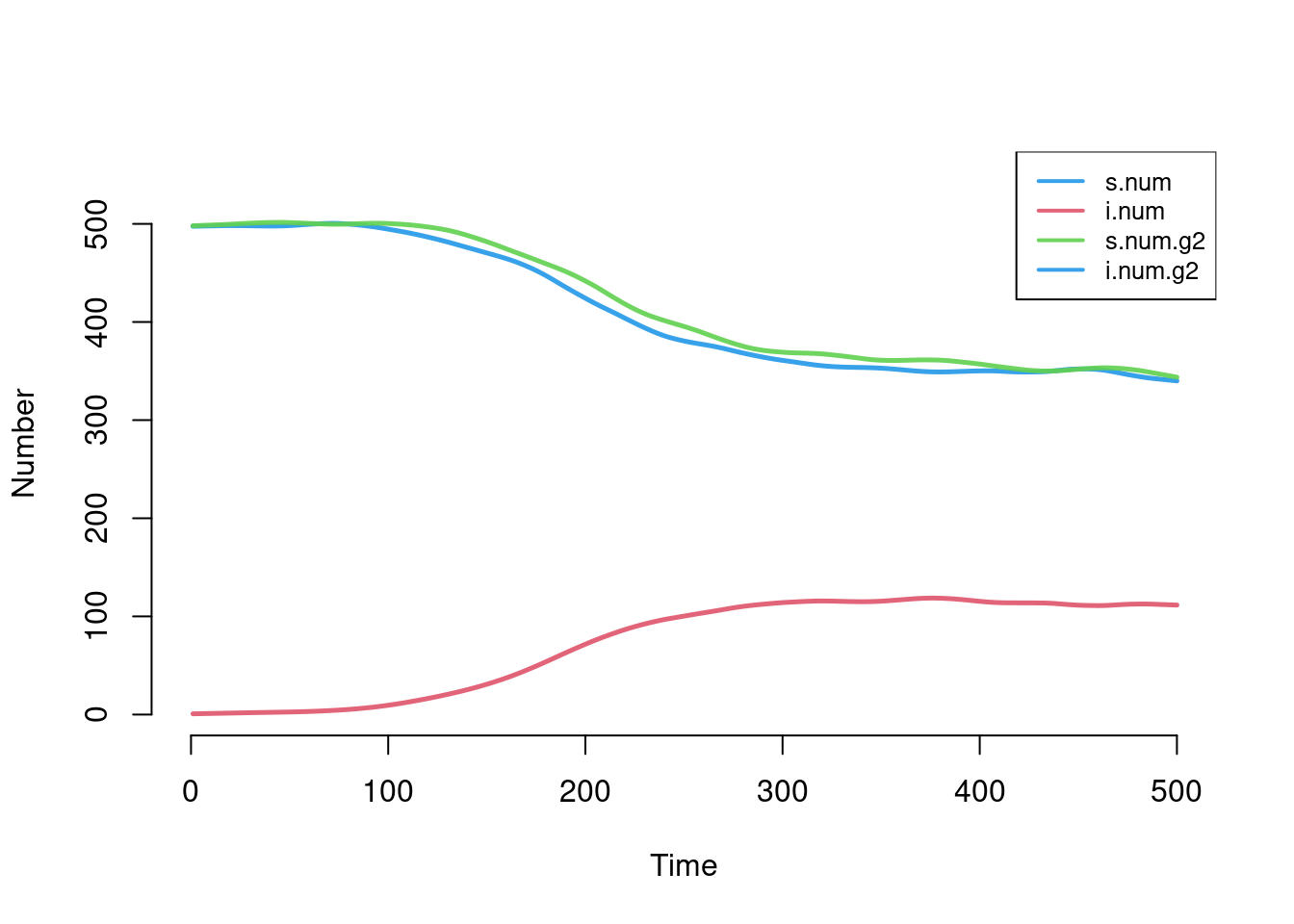
The plot shows a similar disease burden for both groups, with a disease prevalence of around 20% in both groups at time step 400. But we see similar epidemic trajectories for both groups because their transmission probabilities and recovery rates have balanced out: both groups have an \(R_0 = 2.5\).
par(mfrow = c(1,1))
plot(sim)
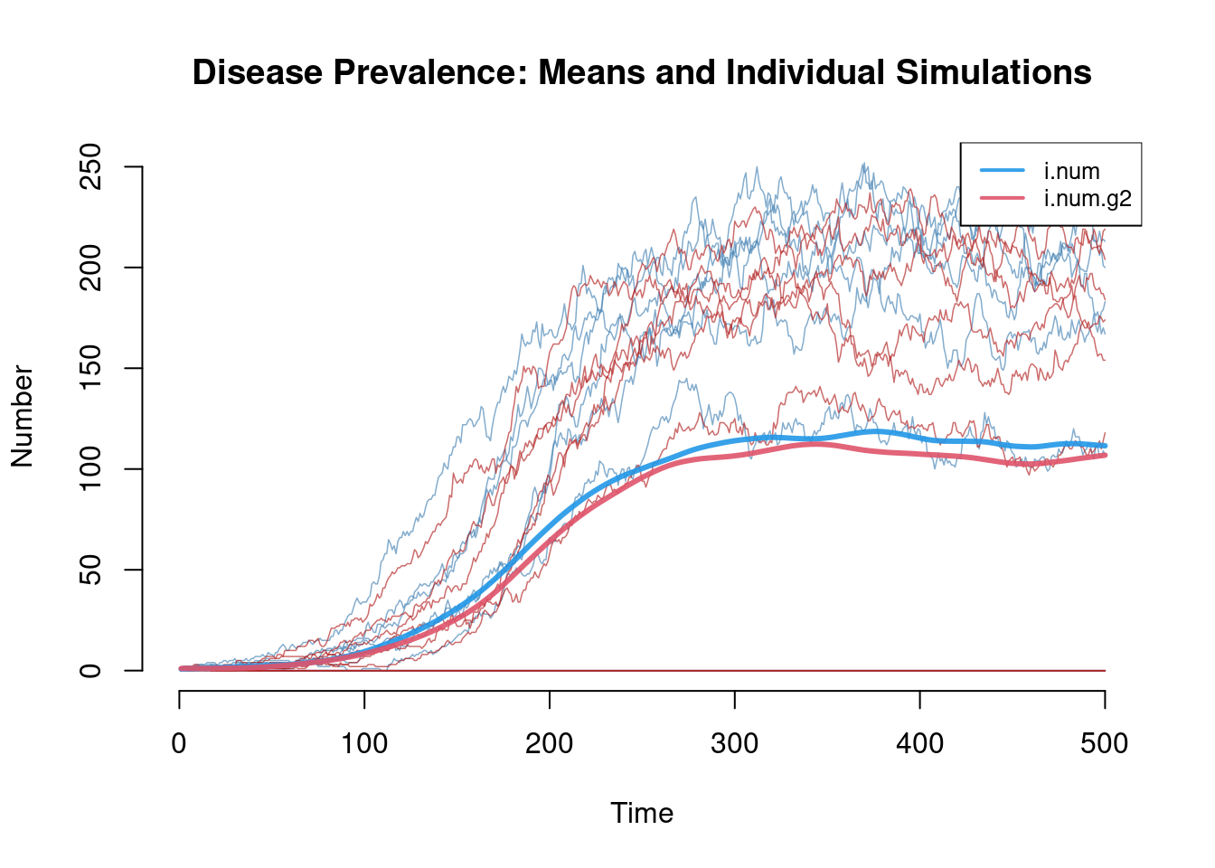
The default plotting options for two-group models will only show the simulation means, so the additional summary information (quantiles and individual simulation lines) must be toggled on as needed. This second plot shows that we must be careful not to look only at the simulation means. In this case, the mean lines are an average of normally occurring epidemics in 6 simulations and extinct epidemics in 4 simulations. Model extinctions occur in this case because the recovery rate in the first group is relatively short and there is only one person initially infected.
plot(sim, y = c("i.num", "i.num.g2"), mean.lwd = 3, sim.lines = TRUE,
     sim.col = c("steelblue", "firebrick"), legend = TRUE,
     main = "Disease Prevalence: Means and Individual Simulations")
Another useful diagnostic for this behavior is found in the summary function, where we would find that at time step 400, the mean number infected is 115.7, and the standard deviation around that mean is 104. If this phenomenon of stochastic model extinction represents the underlying epidemic process of interest in which there is one initial infected, these icm models have utility per se. But if the number of initial infected is arbitrary (or unknown), the model extinctions may be an artificiality to be removed: in that case, one may increase the total population size (specifically the initial number infected) or reduce the size of the time step (and also, adjust the denominators of the parameters with units of time in them).
5.5 Next Steps
This tutorial has provided the basics to get started with exploring ICMs with EpiModel. From here, we suggest that you learn about stochastic modeling of epidemics that incorporates dynamic networks in the Basic Network Models with EpiModel tutorial. This will provide a framework for flexible microsimulation models that expands on the stochastic model approch of ICMs.