Observed Network Layer for Network Epidemic Models

Wraps a fully observed contact network, either a static network or a networkDynamic with edge spells, as a layer that netsim() accepts anywhere in its layer list alongside the layers estimated with netest(). The simulation reads the edges active at each time step from the observed object; there is no formation model, no dissolution model, and no resimulation. It is an addition to netest for the case in which the whole network has been observed, not a substitute for estimation from a sample (see Details).

Usage

netcensus(nw, window = NULL)

Arguments

nw: An object of class network (a static census: the edges are active at every time step) or networkDynamic (a dynamic census: the edges active at time step at are those whose spells cover at). The network must be undirected and not bipartite, without loops or parallel edges (a pair of nodes in contact over several periods has one edge with several activity spells). Vertex attributes on nw are carried into the simulation as nodal attributes, wherever the layer sits in the layer list; temporally extended vertex attributes (*.active) are dropped with a message, since netsim keeps its own disease status.
window: Observation window of a dynamic census, as c(start, end), read like a networkDynamic spell as the half-open interval [start, end): c(1, 11) covers time steps 1 to 10. Defaults to the net.obs.period network attribute when nw has one with finite bounds, and otherwise to the range of the finite edge spell times. Used to summarize the observed edges and to warn when a simulation ends before the window begins or runs past its end.

Value

An object of class netcensus, a list with elements:

newnetwork: the observed network, with temporally extended vertex attributes removed.
dynamic: TRUE for a networkDynamic census, FALSE for a static one.
window: the observation window of a dynamic census, or NULL.
edapprox: FALSE.
summary: a list with the node count, the vertex attribute names, and either the edge count, mean degree, and number of isolates (static) or the number of distinct edges ever observed, the first and last time steps in the window, and the number of edges active at each of those steps, or at 1000 evenly spaced steps for longer windows (dynamic).

Details

netest() exists to turn partial, usually egocentric, network data into a generative model that netsim can simulate from. That is the general workflow, because samples are the norm and the fit is what lets a sample stand in for a population. When the whole network has been observed, for every node and every contact and, for a dynamic census, over every time step, there is nothing to estimate: the observed object is what netsim would otherwise have to generate. netcensus places it in the layer list directly. Sensor, proximity-logger, contact-tracing, and animal-tracking datasets are the usual sources. It is the wrong tool for a sample from which one wants to generalize, and it is not a way to model how the observed ties arise; a network whose ties are to be reproduced from their predictors is estimated with netest, whatever their turnover.

For a networkDynamic census, EpiModel time step at reads the edges active at time at of the observed object, so the simulation clock is the observation clock. A census recorded in other units, such as seconds or calendar dates, needs its spell times rescaled to time steps first. Match the time steps of control.net() to the observation window. Past its end, the layer holds only the edges whose spells extend beyond it: spells censored at the end of the observation (terminus Inf, as in tergm and EpiModel output) stay active, and spells that end with the observation, as in most contact data, leave the layer empty. netsim() warns when the simulation ends before the window begins or nsteps reaches its end. Vertex activity spells are not used; every node is present throughout.

The layer reads the observed object on the simulation clock, so a simulation with a dynamic census layer is restarted from the netsim object itself (selecting a simulation with get_sims()) rather than from make_restart_point(), which re-bases the time steps and stops on such a layer.

A census has a fixed node set, so vital dynamics are refused: netsim() stops when the model has arrivals or departures and a netcensus layer, and arrive_nodes() and depart_nodes() stop if a custom module tries to add or remove nodes. Duration tracking under tergmLite is also refused for a dynamic census, whose observed spells already carry the durations.

The layer is skipped by the network resimulation and the edges correction, and the built-in infection modules read it through discord_edgelist() like any other layer, so per-layer inf.prob and act.rate may be given with multilayer() in param.net(). Under tergmLite, the active edgelist is extracted from the observed object at every time step; without tergmLite, the networkDynamic object is used as stored. Network statistics are recorded through nwstats.formula in control.net(), with the default "formation" meaning ~edges. netdx() refuses a netcensus object, since there is no model to diagnose; print summarizes the observed edges over the window.

Examples

# \donttest{
# A dynamic census: an observed networkDynamic with edge spells, here 80
# contacts between 50 people over 30 time steps
set.seed(4)
pairs <- t(combn(50, 2))[sample.int(choose(50, 2), 80), ]
onset <- sample(0:25, 80, replace = TRUE)
spells <- data.frame(onset = onset,
                     terminus = onset + sample(2:10, 80, replace = TRUE),
                     tail = pairs[, 1], head = pairs[, 2])
nd <- networkDynamic::networkDynamic(base.net = network_initialize(n = 50),
                                     edge.spells = spells)
#> Created net.obs.period to describe network
#>  Network observation period info:
#>   Number of observation spells: 1 
#>   Maximal time range observed: 0 until 35 
#>   Temporal mode: continuous 
#>   Time unit: unknown 
#>   Suggested time increment: NA 
obs <- netcensus(nd, window = c(0, 30))
obs
#> EpiModel Observed Network Layer
#> =======================
#> Model class: netcensus
#> Network type: dynamic (networkDynamic)
#> 
#> Layer Summary
#> -----------------------
#> Nodes: 50
#> Observation window: [0, 30), time steps 0 to 29
#> Edges ever observed: 80
#> Edges active per step: min 2 , median 14 , max 20
#> Mean degree per step: 0.543
#> Vertex attributes: none

param <- param.net(inf.prob = 0.5, act.rate = 1)
init <- init.net(i.num = 5)
control <- control.net(type = "SI", nsteps = 25, nsims = 2,
                       resimulate.network = FALSE, verbose = FALSE)
sim <- netsim(obs, param, init, control)
plot(sim)


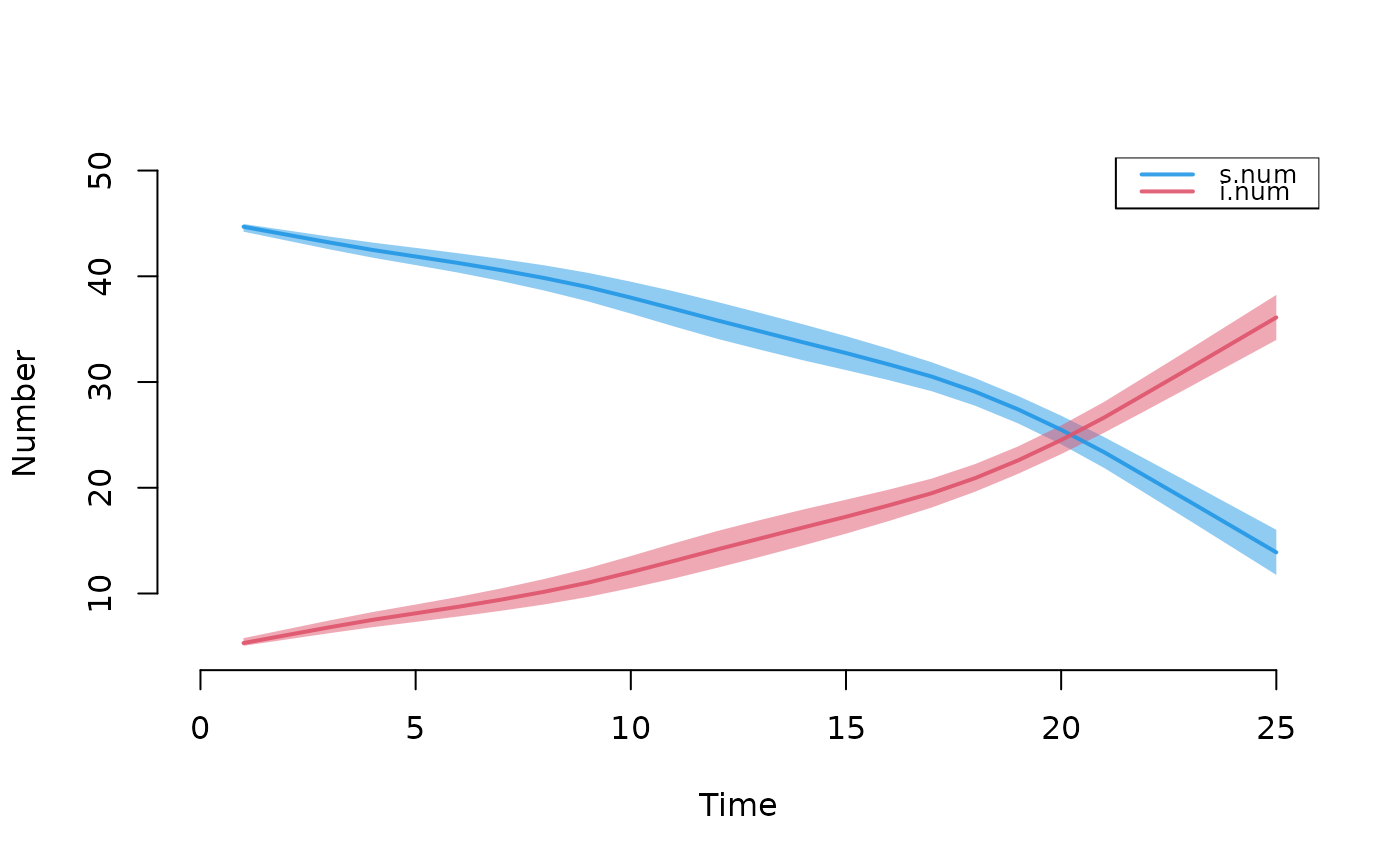# The same census under tergmLite, with the active edges read each step
control <- control.net(type = "SI", nsteps = 25, nsims = 2,
                       tergmLite = TRUE, resimulate.network = TRUE,
                       verbose = FALSE)
sim <- netsim(obs, param, init, control)

# A static census next to an estimated layer
nw <- network_initialize(n = 100)
nw <- add.edges(nw, tail = 1:50, head = 51:100)
est <- netest(nw, ~edges, target.stats = 40,
              coef.diss = dissolution_coefs(~offset(edges), 10),
              verbose = FALSE)
#> Starting simulated annealing (SAN)
#> Iteration 1 of at most 4
#> Finished simulated annealing
#> Starting maximum pseudolikelihood estimation (MPLE):
#> Obtaining the responsible dyads.
#> Evaluating the predictor and response matrix.
#> Maximizing the pseudolikelihood.
#> Finished MPLE.
sim <- netsim(list(netcensus(nw), est),
              param.net(inf.prob = multilayer(0.3, 0.1)),
              init.net(i.num = 5),
              control.net(type = "SI", nsteps = 20, nsims = 1,
                          tergmLite = TRUE, resimulate.network = TRUE,
                          verbose = FALSE))
# }