Dynamic Network Model Diagnostics

Runs diagnostic simulations on an ERGM/STERGM estimated with netest to assess whether the fitted model reproduces the intended network features. Both static (cross-sectional) and dynamic (temporal) diagnostics are supported. This is the recommended second step in the network modeling pipeline, after estimation with netest and before epidemic simulation with netsim.

Usage

netdx(
  x,
  nsims = 1,
  dynamic = TRUE,
  nsteps = NULL,
  nwstats.formula = "formation",
  set.control.ergm = control.simulate.formula(),
  set.control.tergm = control.simulate.formula.tergm(MCMC.maxchanges =
    .Machine$integer.max),
  sequential = TRUE,
  keep.tedgelist = FALSE,
  keep.tnetwork = FALSE,
  verbose = TRUE,
  ncores = 1,
  skip.dissolution = FALSE,
  future.use.plan = FALSE
)

Arguments

x: An EpiModel object of class netest.
nsims: Number of simulations to run. For dynamic diagnostics, 5–10 simulations are usually sufficient to assess model fit. For static diagnostics, use 10,000+ draws to obtain stable estimates.
dynamic: If TRUE, runs dynamic diagnostics that simulate the temporal network forward in time, checking both formation targets and partnership duration/dissolution. If FALSE, draws from the static ERGM fit to check cross-sectional network structure only (faster, but does not verify dissolution dynamics). Static diagnostics are only available when the model was fit with the edges dissolution approximation (edapprox = TRUE in netest).
nsteps: Number of time steps per simulation (dynamic simulations only). Should be at least several multiples of the longest target partnership duration to allow the duration and dissolution statistics to stabilize. For example, if the target duration is 50, running for 500 time steps is a reasonable starting point.
nwstats.formula: A right-hand sided ERGM formula with the network statistics of interest. The default is the formation formula of the network model contained in x. You may track additional network statistics beyond the formation terms by specifying them here, such as ~ edges + meandeg + concurrent + degree(0:4). This is useful for verifying that the model produces reasonable values for network features that were not directly targeted in the formation model.
set.control.ergm: Control arguments passed to ergm's simulate_formula.network (see details).
set.control.tergm: Control arguments passed to tergm's simulate_formula.network (see details).
sequential: For static diagnostics (dynamic=FALSE): if FALSE, each of the nsims simulated Markov chains begins at the initial network; if TRUE, the end of one simulation is used as the start of the next.
keep.tedgelist: If TRUE, keep the timed edgelist generated from the dynamic simulations. Returned in the form of a list of matrices, with one entry per simulation. Accessible at $edgelist.
keep.tnetwork: If TRUE, keep the full networkDynamic objects from the dynamic simulations. Returned in the form of a list of nD objects, with one entry per simulation. Accessible at $network.
verbose: If TRUE, print progress to the console.
ncores: Number of processor cores to run multiple simulations on, using the future framework.
skip.dissolution: If TRUE, skip over the calculations of duration and dissolution stats in netdx.
future.use.plan: If TRUE, netsim will use the user-defined future::plan for its parallelization. Otherwise, multisession is used with workers = ncores.

Value

A list of class netdx. Use print() to view summary tables of formation statistics, duration, and dissolution diagnostics. Use plot.netdx to visualize these diagnostics over time. Use as.data.frame.netdx() to extract timed edgelists (if keep.tedgelist = TRUE).

Details

The netdx function handles dynamic network diagnostics for network models fit with the netest function. Given the fitted model, netdx simulates a specified number of dynamic networks for a specified number of time steps per simulation. The network statistics in nwstats.formula are saved for each time step. Summary statistics for the formation model terms, as well as dissolution model and relational duration statistics, are then calculated and can be accessed when printing or plotting the netdx object. See print.netdx and plot.netdx for details on printing and plotting.

Control Arguments

Models fit with the full STERGM method in netest (setting the edapprox argument to FALSE) require only a call to tergm's simulate_formula.network. Control parameters for those simulations may be set using set.control.tergm in netdx. The parameters should be input through the control.simulate.formula.tergm function, with the available parameters listed in the tergm::control.simulate.formula.tergm help page in the tergm package.

Models fit with the ERGM method with the edges dissolution approximation (setting edapprox to TRUE) require a call first to ergm's simulate_formula.network for simulating an initial network, and second to tergm's simulate_formula.network for simulating that static network forward through time. Control parameters may be set for both processes in netdx. For the first, the parameters should be input through the control.simulate.formula() function, with the available parameters listed in the ergm::control.simulate.formula help page in the ergm package. For the second, parameters should be input through the control.simulate.formula.tergm() function, with the available parameters listed in the tergm::control.simulate.formula.tergm help page in the tergm package. An example is shown below.

Static vs. Dynamic Diagnostics

Static diagnostics (dynamic = FALSE) draw many independent networks from the fitted ERGM and compare the resulting statistics to the target values. This is fast and checks whether the cross-sectional structure is correct, but it does not verify partnership durations or dissolution rates. Dynamic diagnostics (dynamic = TRUE) simulate the full temporal network forward in time, checking both formation targets and dissolution/duration dynamics. Dynamic diagnostics are slower but more comprehensive, and are required to verify models that will be used with vital dynamics (arrivals/departures).

Interpreting Diagnostics

After running netdx, use print() and plot.netdx to inspect the results. Key indicators of a good model fit include:

Formation statistics: The "Sim Mean" should be close to the "Target" value. A small "Pct Diff" (< 5\ indicate good fit.
Duration statistics (dynamic only): The simulated mean edge durations should match the values passed to dissolution_coefs.
Dissolution statistics (dynamic only): The simulated dissolution rates should be approximately 1 / duration.

Common problems: If formation statistics are off, the ERGM may need increased burn-in (via set.control.ergm), or the target statistics may be incompatible (e.g., specifying more edges than the network can support). If durations are off but formation is correct, verify that d.rate was correctly specified in dissolution_coefs for models with vital dynamics.

Examples

# Static diagnostics on a simple model
nw <- network_initialize(n = 100)
formation <- ~edges
target.stats <- 50
coef.diss <- dissolution_coefs(dissolution = ~offset(edges), duration = 25)
est <- netest(nw, formation, target.stats, coef.diss, verbose = FALSE)
#> Starting simulated annealing (SAN)
#> Iteration 1 of at most 4
#> Finished simulated annealing
#> Starting maximum pseudolikelihood estimation (MPLE):
#> Obtaining the responsible dyads.
#> Evaluating the predictor and response matrix.
#> Maximizing the pseudolikelihood.
#> Finished MPLE.
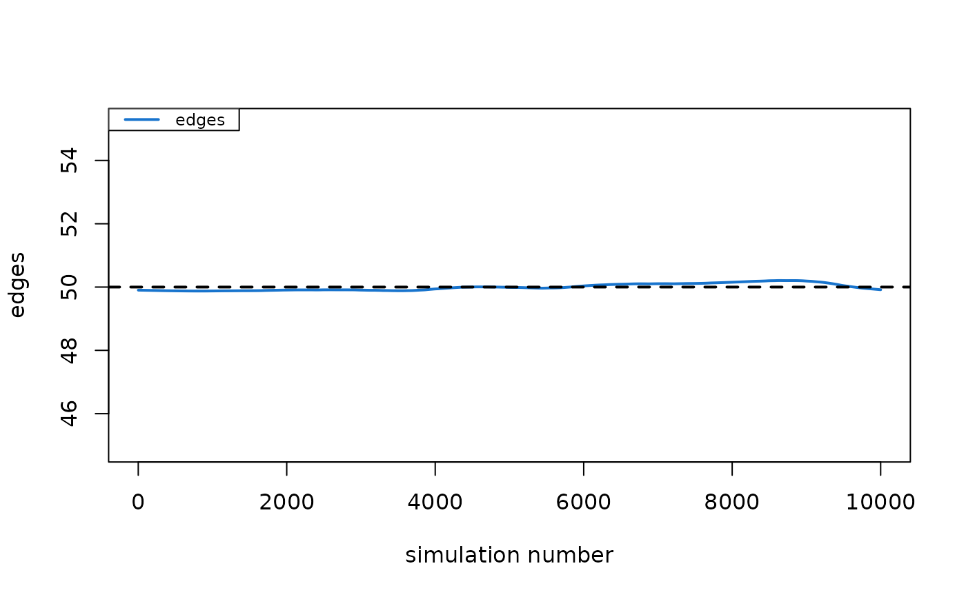
dx <- netdx(est, nsims = 1e4, dynamic = FALSE, verbose = FALSE)
#> Sampling ■■■■■■■■■■■■■■■■■■■■■■■■■■■■■■    96% |  ETA:  0s
dx
#> EpiModel Network Diagnostics
#> =======================
#> Diagnostic Method: Static
#> Simulations: 10000
#> 
#> Formation Diagnostics
#> ----------------------- 
#>       Target Sim Mean Pct Diff Sim SE Z Score SD(Sim Means) SD(Statistic)
#> edges     50   50.009    0.019  0.072   0.131            NA         6.974
plot(dx)


if (FALSE) { # \dontrun{
# Static diagnostics with additional network statistics
dx1 <- netdx(est,
  nsims = 1e4, dynamic = FALSE,
  nwstats.formula = ~ edges + meandeg + concurrent
)
dx1
plot(dx1, method = "b", stats = c("edges", "concurrent"))

# Dynamic diagnostics on the STERGM approximation
dx2 <- netdx(est,
  nsims = 5, nsteps = 500,
  nwstats.formula = ~ edges + meandeg + concurrent,
  set.control.ergm = control.simulate.formula(MCMC.burnin = 1e6)
)
dx2
plot(dx2, stats = c("edges", "meandeg"), plots.joined = FALSE)
plot(dx2, type = "duration")
plot(dx2, type = "dissolution", qnts.col = "orange2")
plot(dx2, type = "dissolution", method = "b", col = "bisque")

# Dynamic diagnostics on a more complex model
nw <- network_initialize(n = 1000)
nw <- set_vertex_attribute(nw, "neighborhood", rep(1:10, 100))
formation <- ~edges + nodematch("neighborhood", diff = TRUE)
target.stats <- c(800, 45, 81, 24, 16, 32, 19, 42, 21, 24, 31)
coef.diss <- dissolution_coefs(dissolution = ~offset(edges) +
                    offset(nodematch("neighborhood", diff = TRUE)),
                    duration = c(52, 58, 61, 55, 81, 62, 52, 64, 52, 68, 58))
est2 <- netest(nw, formation, target.stats, coef.diss, verbose = FALSE)
dx3 <- netdx(est2, nsims = 5, nsteps = 100)
print(dx3)
plot(dx3)
plot(dx3, type = "duration", plots.joined = TRUE, qnts = 0.2, legend = TRUE)
plot(dx3, type = "dissolution", mean.smooth = FALSE, mean.col = "red")
} # }