Working with Model Parameters in EpiModel

Introduction

This vignette assumes familiarity with setting up and running network models in EpiModel. See the Network Modeling for Epidemics (NME) course materials and the EpiModel Gallery for background.

For working with nodal attributes and epidemic summary statistics, see the companion vignette Working with Custom Attributes and Summary Statistics in EpiModel. For network objects and edgelists, see Working with Network Objects in EpiModel.

In a model, parameters are the input variables that define aspects of system behavior. In a basic SIS (Susceptible-Infected-Susceptible) model, these might include an infection probability, an act rate, and a recovery rate. In simple models, each parameter is a single fixed value that remains constant throughout a simulation. Real-world applications, however, often require more flexibility: parameters that change over time (e.g., to represent an intervention rollout or behavioral change during an epidemic), parameters drawn from distributions (for sensitivity analysis or calibration), or large parameter sets managed via spreadsheets.

This vignette demonstrates how to implement:

Scenarios: Named sets of parameter changes applied at the start of a simulation or at specific time steps—the primary mechanism for time-varying parameters, counterfactual analysis, and intervention modeling.
Parameter input via tables: Passing many parameters at once through a data.frame, enabling spreadsheet-based parameter management.
Random parameters: Distributions of parameter values rather than single fixed values, for uncertainty quantification and sensitivity analysis.
Parameter and control updaters (advanced): The low-level mechanism underlying scenarios, exposed directly for cases where the scenario API is not flexible enough.

Scenarios

Scenarios allow you to define named sets of parameter values that can change at specific time steps during a simulation. This is the recommended approach for implementing time-varying parameters—for example, modeling an intervention that reduces transmission probability partway through an epidemic, or comparing multiple policy alternatives.

Our research paper implementing time-varying parameter scenarios for COVID-19 sexual distancing interventions was published in the Journal of Infectious Diseases. The code can be found here.

Setup

First, we set up a simple SIS model as the base case.

set.seed(10)

nw <- network_initialize(n = 200)
est <- netest(nw,
  formation = ~edges, target.stats = 60,
  coef.diss = dissolution_coefs(~offset(edges), 10, 0),  # duration = 10, closed population
  verbose = FALSE
)
#> Starting simulated annealing (SAN)
#> Iteration 1 of at most 4
#> Finished simulated annealing
#> Starting maximum pseudolikelihood estimation (MPLE):
#> Obtaining the responsible dyads.
#> Evaluating the predictor and response matrix.
#> Maximizing the pseudolikelihood.
#> Finished MPLE.

param <- param.net(inf.prob = 0.9, rec.rate = 0.01, act.rate = 2)
init <- init.net(i.num = 10)
control <- control.net(type = "SIS", nsims = 1, nsteps = 250, verbose = FALSE)

Scenario Definitions

Scenarios are defined using create_scenario_list, which takes a specially formatted data.frame as input and outputs a list of scenarios usable by EpiModel. We use tibble::tribble here for readability, but any data.frame constructor works.

library(dplyr)
#> 
#> Attaching package: 'dplyr'
#> The following objects are masked from 'package:stats':
#> 
#>     filter, lag
#> The following objects are masked from 'package:base':
#> 
#>     intersect, setdiff, setequal, union

scenarios.df <- tribble(
  ~.scenario.id, ~.at, ~inf.prob, ~rec.rate,
  "base", 0, 0.9, 0.01,
  "initial_change", 0, 0.2, 0.01,
  "multiple_changes", 0, 0.1, 0.04,
  "multiple_changes", 100, 0.9, 0.01,
  "multiple_changes", 200, 0.1, 0.1
)

knitr::kable(scenarios.df)

.scenario.id	.at	inf.prob	rec.rate
base	0	0.9	0.01
initial_change	0	0.2	0.01
multiple_changes	0	0.1	0.04
multiple_changes	100	0.9	0.01
multiple_changes	200	0.1	0.10

The data.frame requires two columns:

.scenario.id: an identifier for the scenario.
.at: the time step at which the parameter changes should apply. Use 0 for changes that take effect before the simulation begins.

Remaining columns are parameter names. They must start with a letter and contain only letters, numbers, or . (underscores are reserved for vector indexing, described below). If a cell is NA, EpiModel sets that parameter to NA—it does not mean “leave unchanged.”

In this example, the "multiple_changes" scenario has three rows sharing the same .scenario.id, representing a single scenario with parameter changes at three different time points.

To convert from the data.frame to a usable list of scenarios:

scenarios.list <- create_scenario_list(scenarios.df)
str(scenarios.list, max.level = 2)
#> List of 3
#>  $ base            :List of 2
#>   ..$ id                 : chr "base"
#>   ..$ .param.updater.list:List of 1
#>  $ initial_change  :List of 2
#>   ..$ id                 : chr "initial_change"
#>   ..$ .param.updater.list:List of 1
#>  $ multiple_changes:List of 2
#>   ..$ id                 : chr "multiple_changes"
#>   ..$ .param.updater.list:List of 3

Running Scenarios

We loop over all scenarios, using use_scenario to create a modified parameter object for each. Under the hood, use_scenario generates parameter updaters (described in the Advanced section below) that apply the specified changes at the designated time steps.

# List to hold simulation results
d_list <- vector(mode = "list", length = length(scenarios.list))
names(d_list) <- names(scenarios.list)

for (scenario in scenarios.list) {
  print(scenario$id)
  sc.param <- use_scenario(param, scenario)
  sim <- netsim(est, sc.param, init, control)
  d_sim <- as.data.frame(sim)
  d_sim[["scenario"]] <- scenario$id
  d_list[[scenario$id]] <- d_sim
}
#> [1] "base"
#> [1] "initial_change"
#> [1] "multiple_changes"
#> 
#>  A MESSAGE occured in module 'epimodel.internal' at step 100
#> 
#> 
#> At timestep = 100 the following parameters were modified:
#> 'inf.prob', 'rec.rate'
#> 
#>  A MESSAGE occured in module 'epimodel.internal' at step 200
#> 
#> 
#> At timestep = 200 the following parameters were modified:
#> 'inf.prob', 'rec.rate'

For the "multiple_changes" scenario, messages appear at time steps 100 and 200 indicating that parameters were modified during the simulation. The other scenarios are silent because their changes occur before the simulation begins (.at = 0).

Now we can plot the results. We use base R plotting here rather than plot.netsim() because we need to overlay results from separate netsim runs on a single axis.

plot(d_list$base$time, d_list$base$i.num,
     type = "l", col = 1, lwd = 2, ylim = c(0, 250),
     xlab = "Time Step", ylab = "Number Infected")
lines(d_list$initial_change$time, d_list$initial_change$i.num,
      type = "l", col = 2, lwd = 2)
lines(d_list$multiple_changes$time, d_list$multiple_changes$i.num,
      type = "l", col = 3, lwd = 2)
abline(v = c(100, 200), lty = 2)
legend("topleft", legend = names(d_list),
       col = 1:3, lwd = 2, cex = 0.9, bty = "n")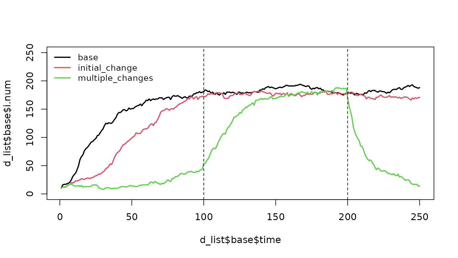

The "initial_change" scenario shows a slower epidemic than the base case because the infection probability is reduced from 0.9 to 0.2 from the start.

The "multiple_changes" scenario demonstrates three phases:

Steps 1–99: Slow growth (low infection probability, higher recovery rate).
Steps 100–199: Base-case parameters applied, so the epidemic trajectory accelerates.
Steps 200–250: Infection probability drops and recovery rate increases, driving rapid epidemic decline.

Scenarios with Parameter Vectors

In full-scale modeling projects, parameters are often vectors. For example, hiv.test.rate might be a vector of length 3 containing weekly HIV screening probabilities for Black, Hispanic, and White persons.

To use vectors in scenarios, create a separate column for each element using the naming convention paramname_N, where N is the position in the vector:

scenarios.df <- tribble(
  ~.scenario.id, ~.at, ~hiv.test.rate_1, ~hiv.test.rate_2, ~hiv.test.rate_3,
  "base", 0, 0.001, 0.001, 0.001,
  "initial_change", 0, 0.002, 0.001, 0.002,
  "multiple_changes", 0, 0.002, 0.001, 0.002,
  "multiple_changes", 100, 0.004, 0.001, 0.004,
  "multiple_changes", 200, 0.008, 0.001, 0.008
)
knitr::kable(scenarios.df)

.scenario.id	.at	hiv.test.rate_1	hiv.test.rate_2	hiv.test.rate_3
base	0	0.001	0.001	0.001
initial_change	0	0.002	0.001	0.002
multiple_changes	0	0.002	0.001	0.002
multiple_changes	100	0.004	0.001	0.004
multiple_changes	200	0.008	0.001	0.008

All elements of a vector parameter must be specified in the data.frame, even if some values do not change across scenarios (e.g., hiv.test.rate_2 is constant here but must still be included).

When working with many parameters, we recommend storing the scenarios.df as a CSV, RDS or Excel file for easier sharing and editing.

# CSV
write.csv(scenarios.df, "scenarios.csv", row.names = FALSE)
scenarios.df <- read.csv("scenarios.csv")

# RDS
saveRDS(scenarios.df, "scenarios.rds")
scenarios.df <- readRDS("scenarios.rds")

Parameter Input via Table

The param.net function accepts a data.frame of parameters through the data.frame.params argument. This allows passing many parameters at once or working with a spreadsheet to track and update parameters before use in EpiModel.

The data.frame requires three columns:

param: The parameter name. For vector parameters (length > 1), append the position with an underscore (e.g., "p_1", "p_2").
value: The parameter value (as a character string).
type: The type of the parameter value. Only three values are accepted: "numeric", "logical", or "character".

Additional columns (e.g., details, source) may be included for documentation but are ignored by EpiModel.

df_params <- tribble(
  ~param, ~value, ~type,
  "hiv.test.rate_1",  "0.003",        "numeric",
  "hiv.test.rate_2",  "0.102",        "numeric",
  "hiv.test.rate_3",  "0.492",        "numeric",
  "prep.require.lnt", "TRUE",         "logical",
  "group_1",          "first",        "character",
  "group_2",          "second",       "character"
)
knitr::kable(df_params)

param	value	type
hiv.test.rate_1	0.003	numeric
hiv.test.rate_2	0.102	numeric
hiv.test.rate_3	0.492	numeric
prep.require.lnt	TRUE	logical
group_1	first	character
group_2	second	character

Pass the table via data.frame.params. These parameters can be combined with named parameters for maximum flexibility. In case of conflict, named parameters take priority over those in the data.frame:

param <- param.net(data.frame.params = df_params,
                   other.param = c(5, 10), act.rate = 1)
param
#> Fixed Parameters
#> ---------------------------
#> hiv.test.rate = 0.003 0.102 0.492
#> prep.require.lnt = TRUE
#> group = first second
#> act.rate = 1
#> other.param = 5 10

Random Parameters

Fixed parameters assume that each input value is known with certainty. In practice, we may want to explore how uncertainty in parameter values propagates to uncertainty in epidemic outcomes. EpiModel supports drawing parameter values from distributions, so that each simulation uses a different realization.

The Model

We demonstrate with a simple SI model.

nw <- network_initialize(n = 50)

est <- netest(
  nw, formation = ~edges,
  target.stats = 25,
  coef.diss = dissolution_coefs(~offset(edges), 10, 0),  # duration = 10, closed population
  verbose = FALSE
)
#> Starting simulated annealing (SAN)
#> Iteration 1 of at most 4
#> Finished simulated annealing
#> Starting maximum pseudolikelihood estimation (MPLE):
#> Obtaining the responsible dyads.
#> Evaluating the predictor and response matrix.
#> Maximizing the pseudolikelihood.
#> Finished MPLE.

param <- param.net(
  inf.prob = 0.3,
  act.rate = 0.5,
  dummy.param = 4,
  dummy.strat.param = c(0, 1)
)

init <- init.net(i.num = 10)
control <- control.net(type = "SI", nsims = 1, nsteps = 5, verbose = FALSE)
mod <- netsim(est, param, init, control)
mod
#> EpiModel Simulation
#> =======================
#> Model class: netsim
#> 
#> Simulation Summary
#> -----------------------
#> Model type: SI
#> No. simulations: 1
#> No. time steps: 5
#> No. NW groups: 1
#> 
#> Fixed Parameters
#> ---------------------------
#> inf.prob = 0.3
#> act.rate = 0.5
#> dummy.param = 4
#> dummy.strat.param = 0 1
#> groups = 1
#> 
#> Model Output
#> -----------------------
#> Variables: s.num i.num num si.flow
#> Networks: sim1
#> Transmissions: sim1
#> 
#> Formation Statistics
#> ----------------------- 
#>       Target Sim Mean Pct Diff Sim SE Z Score SD(Sim Means) SD(Statistic)
#> edges     25     16.8    -32.8  1.114  -7.364            NA          2.49
#> 
#> 
#> Duration Statistics
#> ----------------------- 
#>       Target Sim Mean Pct Diff Sim SE Z Score SD(Sim Means) SD(Statistic)
#> edges     10    8.697  -13.032   0.27  -4.819            NA         0.605
#> 
#> Dissolution Statistics
#> ----------------------- 
#>       Target Sim Mean Pct Diff Sim SE Z Score SD(Sim Means) SD(Statistic)
#> edges    0.1    0.065  -34.615  0.022  -1.608            NA         0.048

Here we define four parameters: inf.prob (which will remain fixed), act.rate, dummy.param, and dummy.strat.param (which we will make random below). The dummy.strat.param parameter is a vector of length 2, which could represent a parameter stratified by subpopulation.

Adding Random Parameters

To draw parameters from distributions, use the random.params argument to param.net. There are two approaches.

Generator Functions

Define a generator function for each random parameter:

my.randoms <- list(
  act.rate = param_random(c(0.25, 0.5, 0.75)),
  dummy.param = function() rbeta(1, 1, 2),
  dummy.strat.param = function() {
    c(rnorm(1, 0.05, 0.01),
      rnorm(1, 0.15, 0.03))
  }
)

param <- param.net(
  inf.prob = 0.3,
  random.params = my.randoms
)

param
#> Fixed Parameters
#> ---------------------------
#> inf.prob = 0.3
#> 
#> Random Parameters
#> (Not drawn yet)
#> ---------------------------
#> act.rate = <function>
#> dummy.param = <function>
#> dummy.strat.param = <function>

The my.randoms list contains three elements:

act.rate uses the param_random function factory provided by EpiModel (see ?param_random). Each simulation samples one of the three values with equal probability.
dummy.param is a zero-argument function that returns a single draw from a Beta(1, 2) distribution.
dummy.strat.param is a zero-argument function that returns a vector of length 2, each element drawn from a normal distribution with different mean and standard deviation.

Each element must be named after the parameter it fills and must be a function taking no arguments, returning a vector of the correct length for that parameter. When we print the parameter list before running the model, random parameters appear as function definitions since their values have not yet been realized.

control <- control.net(type = "SI", nsims = 3, nsteps = 5, verbose = FALSE)
mod <- netsim(est, param, init, control)

mod
#> EpiModel Simulation
#> =======================
#> Model class: netsim
#> 
#> Simulation Summary
#> -----------------------
#> Model type: SI
#> No. simulations: 3
#> No. time steps: 5
#> No. NW groups: 1
#> 
#> Fixed Parameters
#> ---------------------------
#> inf.prob = 0.3
#> groups = 1
#> 
#> Random Parameters
#> ---------------------------
#> act.rate = 0.5 0.75 0.25
#> dummy.param = 0.5293276 0.2734432 0.11582
#> dummy.strat.param = <list>
#> 
#> Model Output
#> -----------------------
#> Variables: s.num i.num num si.flow
#> Networks: sim1 ... sim3
#> Transmissions: sim1 ... sim3
#> 
#> Formation Statistics
#> ----------------------- 
#>       Target Sim Mean Pct Diff Sim SE Z Score SD(Sim Means) SD(Statistic)
#> edges     25   21.667  -13.333  1.022  -3.262          4.46         3.958
#> 
#> 
#> Duration Statistics
#> ----------------------- 
#>       Target Sim Mean Pct Diff Sim SE Z Score SD(Sim Means) SD(Statistic)
#> edges     10    8.977  -10.226  0.387  -2.642         1.593         1.499
#> 
#> Dissolution Statistics
#> ----------------------- 
#>       Target Sim Mean Pct Diff Sim SE Z Score SD(Sim Means) SD(Statistic)
#> edges    0.1    0.114   13.774  0.015   0.938         0.029         0.057

After running 3 simulations, inf.prob remains under “Fixed Parameters” while the random parameters each have 3 realized values (one per simulation). The vector parameter dummy.strat.param shows <list> because each realization is itself a vector of length 2.

To inspect the realized values:

all.params <- get_param_set(mod)
all.params
#>   sim inf.prob vital groups act.rate dummy.param dummy.strat.param_1
#> 1   1      0.3 FALSE      1     0.50   0.5293276          0.05392462
#> 2   2      0.3 FALSE      1     0.75   0.2734432          0.04759042
#> 3   3      0.3 FALSE      1     0.25   0.1158200          0.05619374
#>   dummy.strat.param_2
#> 1           0.1511654
#> 2           0.1293028
#> 3           0.1918158

These can be merged with epidemic output for analysis of parameter-outcome relationships:

epi <- as.data.frame(mod)
left_join(epi, all.params)
#> Joining with `by = join_by(sim)`
#>    sim time s.num i.num num si.flow inf.prob vital groups act.rate dummy.param
#> 1    1    1    40    10  50      NA      0.3 FALSE      1     0.50   0.5293276
#> 2    1    2    40    10  50       0      0.3 FALSE      1     0.50   0.5293276
#> 3    1    3    36    14  50       4      0.3 FALSE      1     0.50   0.5293276
#> 4    1    4    34    16  50       2      0.3 FALSE      1     0.50   0.5293276
#> 5    1    5    34    16  50       0      0.3 FALSE      1     0.50   0.5293276
#> 6    2    1    40    10  50      NA      0.3 FALSE      1     0.75   0.2734432
#> 7    2    2    39    11  50       1      0.3 FALSE      1     0.75   0.2734432
#> 8    2    3    38    12  50       1      0.3 FALSE      1     0.75   0.2734432
#> 9    2    4    36    14  50       2      0.3 FALSE      1     0.75   0.2734432
#> 10   2    5    36    14  50       0      0.3 FALSE      1     0.75   0.2734432
#> 11   3    1    40    10  50      NA      0.3 FALSE      1     0.25   0.1158200
#> 12   3    2    40    10  50       0      0.3 FALSE      1     0.25   0.1158200
#> 13   3    3    40    10  50       0      0.3 FALSE      1     0.25   0.1158200
#> 14   3    4    40    10  50       0      0.3 FALSE      1     0.25   0.1158200
#> 15   3    5    39    11  50       1      0.3 FALSE      1     0.25   0.1158200
#>    dummy.strat.param_1 dummy.strat.param_2
#> 1           0.05392462           0.1511654
#> 2           0.05392462           0.1511654
#> 3           0.05392462           0.1511654
#> 4           0.05392462           0.1511654
#> 5           0.05392462           0.1511654
#> 6           0.04759042           0.1293028
#> 7           0.04759042           0.1293028
#> 8           0.04759042           0.1293028
#> 9           0.04759042           0.1293028
#> 10          0.04759042           0.1293028
#> 11          0.05619374           0.1918158
#> 12          0.05619374           0.1918158
#> 13          0.05619374           0.1918158
#> 14          0.05619374           0.1918158
#> 15          0.05619374           0.1918158

Parameter Sets

Generator functions draw each parameter independently. When parameters need to be correlated—for example, when using Latin hypercube sampling or when one parameter is derived from another—use pre-defined parameter sets instead.

Define a data.frame where each row is a complete set of correlated parameter values:

n <- 5

related.param <- data.frame(
  dummy.param = rbeta(n, 1, 2)
)

related.param$dummy.strat.param_1 <- related.param$dummy.param + rnorm(n)
related.param$dummy.strat.param_2 <- related.param$dummy.param * 2 + rnorm(n)

related.param
#>   dummy.param dummy.strat.param_1 dummy.strat.param_2
#> 1  0.40042189           1.6831189           1.0748786
#> 2  0.73021770           2.3839536           1.3420617
#> 3  0.05306671           0.6405278          -0.7281755
#> 4  0.90490846          -1.3179645          -0.4500947
#> 5  0.48049243           0.7020599           2.3109663

Each row contains parameter values that will be used together in a single simulation. Vector parameters use the same paramname_N suffix convention as scenarios. This means underscores are reserved and cannot appear in parameter names themselves.

Save the parameter set in the my.randoms list under the reserved name param.random.set:

my.randoms <- list(
  act.rate = param_random(c(0.25, 0.5, 0.75)),
  param.random.set = related.param
)

param <- param.net(
  inf.prob = 0.3,
  random.params = my.randoms
)

param
#> Fixed Parameters
#> ---------------------------
#> inf.prob = 0.3
#> 
#> Random Parameters
#> (Not drawn yet)
#> ---------------------------
#> act.rate = <function>
#> param.random.set = <data.frame> ( dimensions: 5 3 )

The inf.prob parameter remains fixed, act.rate remains independently random, and the two remaining parameters are drawn as correlated sets from the data.frame.

control <- control.net(type = "SI", nsims = 3, nsteps = 5, verbose = FALSE)
mod <- netsim(est, param, init, control)

mod
#> EpiModel Simulation
#> =======================
#> Model class: netsim
#> 
#> Simulation Summary
#> -----------------------
#> Model type: SI
#> No. simulations: 3
#> No. time steps: 5
#> No. NW groups: 1
#> 
#> Fixed Parameters
#> ---------------------------
#> inf.prob = 0.3
#> groups = 1
#> 
#> Random Parameters
#> ---------------------------
#> dummy.param = 0.9049085 0.4804924 0.4004219
#> dummy.strat.param = <list>
#> act.rate = 0.75 0.75 0.75
#> 
#> Model Output
#> -----------------------
#> Variables: s.num i.num num si.flow
#> Networks: sim1 ... sim3
#> Transmissions: sim1 ... sim3
#> 
#> Formation Statistics
#> ----------------------- 
#>       Target Sim Mean Pct Diff Sim SE Z Score SD(Sim Means) SD(Statistic)
#> edges     25   25.933    3.733  0.502   1.859         0.757         1.944
#> 
#> 
#> Duration Statistics
#> ----------------------- 
#>       Target Sim Mean Pct Diff Sim SE Z Score SD(Sim Means) SD(Statistic)
#> edges     10    9.584   -4.158  0.183  -2.275          0.68         0.708
#> 
#> Dissolution Statistics
#> ----------------------- 
#>       Target Sim Mean Pct Diff Sim SE Z Score SD(Sim Means) SD(Statistic)
#> edges    0.1    0.114    14.49  0.011    1.27         0.022         0.044

Verify that correlated sets are sampled together:

related.param
#>   dummy.param dummy.strat.param_1 dummy.strat.param_2
#> 1  0.40042189           1.6831189           1.0748786
#> 2  0.73021770           2.3839536           1.3420617
#> 3  0.05306671           0.6405278          -0.7281755
#> 4  0.90490846          -1.3179645          -0.4500947
#> 5  0.48049243           0.7020599           2.3109663
get_param_set(mod)
#>   sim inf.prob vital groups dummy.param dummy.strat.param_1 dummy.strat.param_2
#> 1   1      0.3 FALSE      1   0.9049085          -1.3179645          -0.4500947
#> 2   2      0.3 FALSE      1   0.4804924           0.7020599           2.3109663
#> 3   3      0.3 FALSE      1   0.4004219           1.6831189           1.0748786
#>   act.rate
#> 1     0.75
#> 2     0.75
#> 3     0.75

Time-Varying Parameters and Control Settings (Advanced)

The scenarios system described above uses an internal updater module to implement parameter changes at designated time steps. This section describes the underlying updater mechanism directly. Use this when the scenario API is not flexible enough—for example, when you need relative (function-based) parameter changes or time-varying control settings.

Parameter Updaters

An updater is a list with two required elements: at (the time step for the change) and param (a named list of new parameter values):

list(
  at = 10,
  param = list(
    inf.prob = 0.3,
    act.rate = 0.5
  )
)
#> $at
#> [1] 10
#> 
#> $param
#> $param$inf.prob
#> [1] 0.3
#> 
#> $param$act.rate
#> [1] 0.5

This updater sets inf.prob to 0.3 and act.rate to 0.5 at time step 10. Multiple updaters are combined in a list:

list.of.updaters <- list(
  list(
    at = 100,
    param = list(
      inf.prob = 0.3,
      act.rate = 0.3
    )
  ),
  list(
    at = 125,
    param = list(
      inf.prob = 0.01
    )
  )
)

Incorporating Updaters

Pass the updater list to param.net via the .param.updater.list argument:

param <- param.net(
 inf.prob = 0.1,
 act.rate = 0.1,
 .param.updater.list = list.of.updaters
)
init <- init.net(i.num = 10)
control <- control.net(
 type = "SI",
 nsims = 1,
 nsteps = 200,
 verbose = FALSE
)

nw <- network_initialize(n = 100)
est <- netest(
  nw,
  formation = ~edges,
  target.stats = 50,
  coef.diss = dissolution_coefs(~offset(edges), 10, 0),  # duration = 10, closed population
  verbose = FALSE
)
#> Starting simulated annealing (SAN)
#> Iteration 1 of at most 4
#> Finished simulated annealing
#> Starting maximum pseudolikelihood estimation (MPLE):
#> Obtaining the responsible dyads.
#> Evaluating the predictor and response matrix.
#> Maximizing the pseudolikelihood.
#> Finished MPLE.
mod <- netsim(est, param, init, control)
#> 
#>  A MESSAGE occured in module 'epimodel.internal' at step 100
#> 
#> 
#> At timestep = 100 the following parameters were modified:
#> 'inf.prob', 'act.rate'
#> 
#>  A MESSAGE occured in module 'epimodel.internal' at step 125
#> 
#> 
#> At timestep = 125 the following parameters were modified:
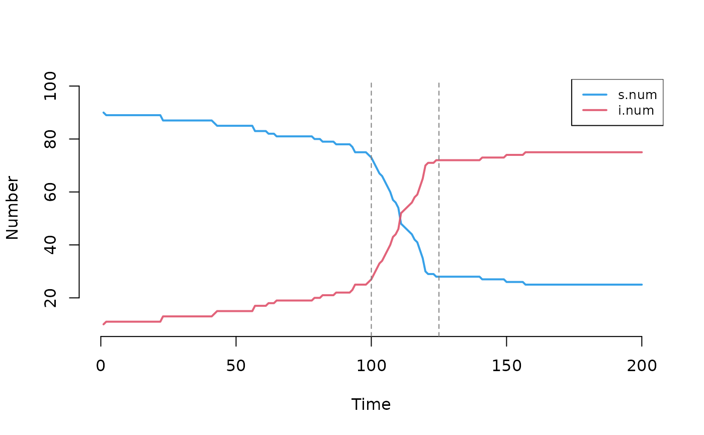
#> 'inf.prob'

The plot shows inflection points at the two parameter change points. At step 100, both inf.prob and act.rate increase from 0.1 to 0.3, accelerating transmission. At step 125, inf.prob drops to 0.01, slowing the epidemic.

plot(mod, mean.smooth = FALSE)
abline(v = c(100, 125), lty = 2, col = "grey50")

Verbosity

Each updater can include an optional verbose element. When TRUE (the default), EpiModel prints a message describing the changes:

list(
  at = 10,
  param = list(
    inf.prob = 0.3,
    act.rate = 0.5
  ),
  verbose = TRUE
)
#> $at
#> [1] 10
#> 
#> $param
#> $param$inf.prob
#> [1] 0.3
#> 
#> $param$act.rate
#> [1] 0.5
#> 
#> 
#> $verbose
#> [1] TRUE

Relative Parameter Changes

Instead of setting a parameter to a fixed new value, you can define a function that transforms the current value. This is useful for multiplicative changes or logit-scale adjustments.

list(
  at = 10,
  param = list(
    inf.prob = function(x) plogis(qlogis(x) + log(2)),
    act.rate = 0.5
  )
)
#> $at
#> [1] 10
#> 
#> $param
#> $param$inf.prob
#> function (x) 
#> plogis(qlogis(x) + log(2))
#> 
#> $param$act.rate
#> [1] 0.5

In this updater, act.rate is set to the fixed value 0.5 as before. For inf.prob, instead of a value, we provide a function. At time step 10, EpiModel applies this function to the current value of inf.prob. If inf.prob was set to 0.1 by param.net, the function computes plogis(qlogis(0.1) + log(2)) = 0.1818, which doubles the odds of transmission while keeping the result on the probability scale.

Time-Varying Control Settings

Control settings can also be changed during a simulation using the same updater mechanism. Each control updater uses a control element (instead of param):

list.of.updaters <- list(
  list(
    at = 100,
    control = list(
      resimulate.network = FALSE
    )
  ),
  list(
    at = 125,
    control = list(
      verbose = FALSE
    )
  )
)

This example turns off network resimulation at step 100 and disables model verbosity at step 125.

Pass control updaters to control.net via .control.updater.list, paralleling how parameter updaters are passed to param.net via .param.updater.list:

control <- control.net(
 type = "SI",
 nsims = 1,
 nsteps = 200,
 verbose = TRUE,
 .control.updater.list = list.of.updaters
)

EpiModel v2.6.1

2026-04-18