Truncate Simulation Time Series

Left-truncates simulation epidemiological summary statistics and network statistics at a specified time step.

Usage

truncate_sim(x, at, reset.time)

# S3 method for class 'dcm'
truncate_sim(x, at, reset.time = TRUE)

# S3 method for class 'icm'
truncate_sim(x, at, reset.time = TRUE)

# S3 method for class 'netsim'
truncate_sim(x, at, reset.time = TRUE)

Arguments

x

Object of class dcm, netsim, or icm.

at

Time step at which to left-truncate the time series.

reset.time

If TRUE, the time step sequence in the truncated model will be reset to start at 1. If FALSE, the original time step values will be preserved. Default is TRUE.

Value

The updated object of class dcm, netsim, or icm.

Details

This function would be used when running a follow-up simulation from time steps b to c after a burn-in period from time a to b, where the final time window of interest for data analysis is b to c only.

Examples

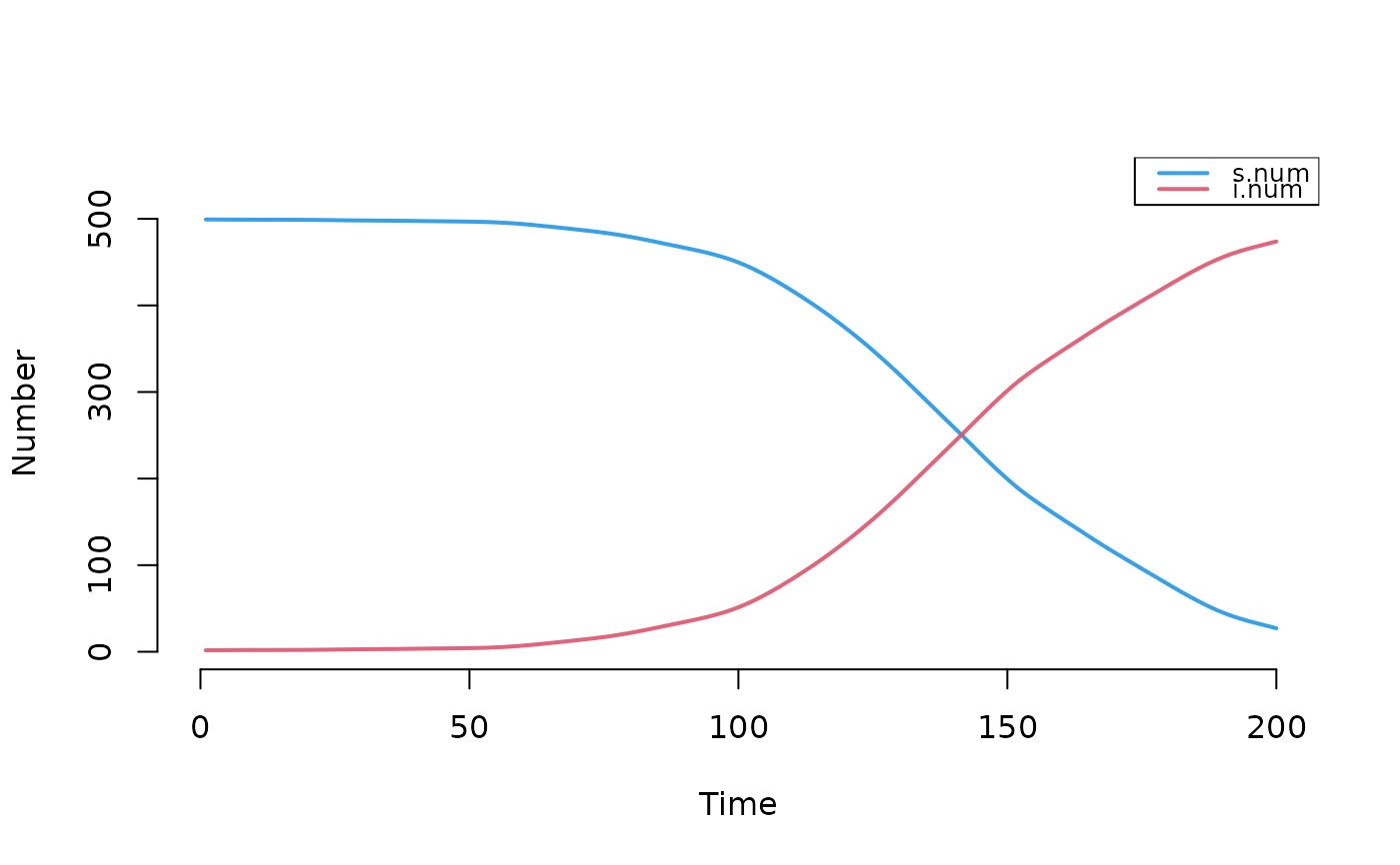
# DCM examples
param <- param.dcm(inf.prob = 0.2, act.rate = 0.25)
init <- init.dcm(s.num = 500, i.num = 1)
control <- control.dcm(type = "SI", nsteps = 200)
mod1 <- dcm(param, init, control)
plot(mod1)


# Reset time
mod2a <- truncate_sim(mod1, at = 150)
plot(mod2a)

head(as.data.frame(mod2a))
#>   time     s.num    i.num  si.flow num
#> 1    1 112.84477 388.1552 4.311259 501
#> 2    2 108.53351 392.4665 4.190824 501
#> 3    3 104.34268 396.6573 4.070347 501
#> 4    4 100.27233 400.7277 3.950123 501
#> 5    5  96.32221 404.6778 3.830429 501
#> 6    6  92.49178 408.5082 3.711522 501

# Do not reset time
mod2b <- truncate_sim(mod1, at = 150, reset.time = FALSE)
plot(mod2b)

head(as.data.frame(mod2b))
#>   time     s.num    i.num  si.flow num
#> 1  150 112.84477 388.1552 4.311259 501
#> 2  151 108.53351 392.4665 4.190824 501
#> 3  152 104.34268 396.6573 4.070347 501
#> 4  153 100.27233 400.7277 3.950123 501
#> 5  154  96.32221 404.6778 3.830429 501
#> 6  155  92.49178 408.5082 3.711522 501

# ICM example
param <- param.icm(inf.prob = 0.2, act.rate = 0.25)
init <- init.icm(s.num = 500, i.num = 1)
control <- control.icm(type = "SI", nsteps = 200, nsims = 1)
mod1 <- icm(param, init, control)

# Reset time
mod2a <- truncate_sim(mod1, at = 150)
plot(mod2a)

head(as.data.frame(mod2a))
#>   sim time s.num i.num num si.flow
#> 1   1    1   145   356 501       7
#> 2   1    2   136   365 501       9
#> 3   1    3   131   370 501       5
#> 4   1    4   130   371 501       1
#> 5   1    5   124   377 501       6
#> 6   1    6   117   384 501       7

# Do not reset time
mod2b <- truncate_sim(mod1, at = 150, reset.time = FALSE)
plot(mod2b)

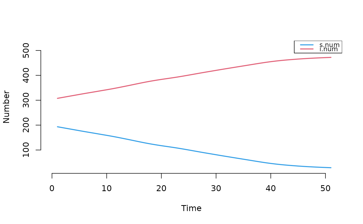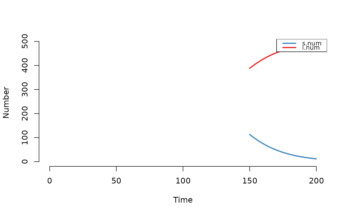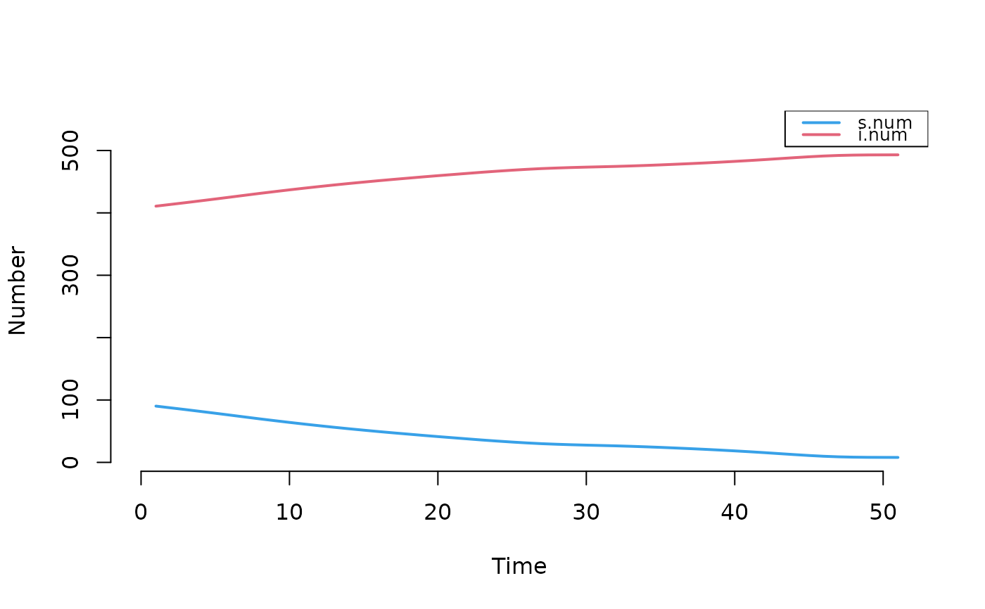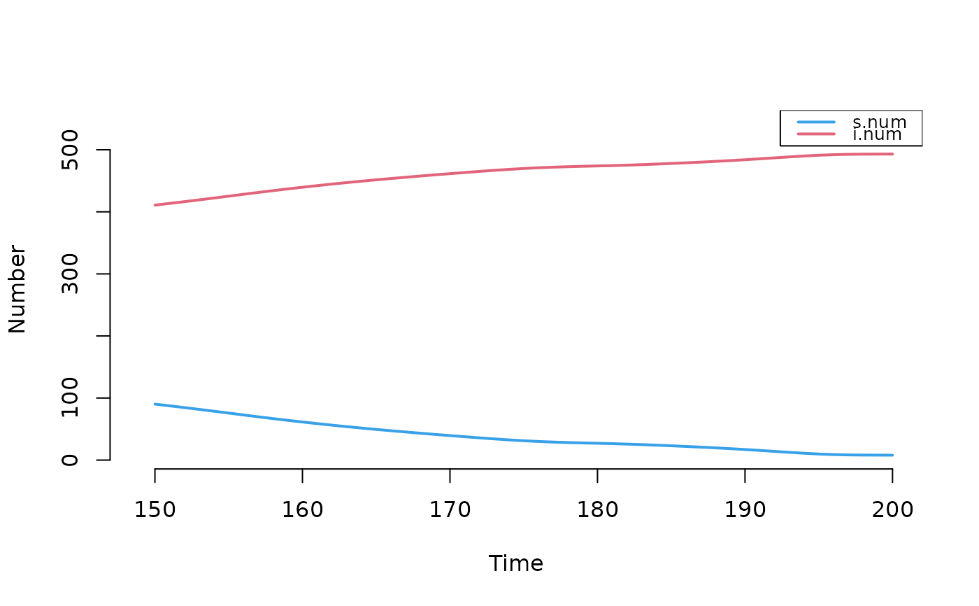head(as.data.frame(mod2b))
#>   sim time s.num i.num num si.flow
#> 1   1  150   145   356 501       7
#> 2   1  151   136   365 501       9
#> 3   1  152   131   370 501       5
#> 4   1  153   130   371 501       1
#> 5   1  154   124   377 501       6
#> 6   1  155   117   384 501       7