Exercise 4: The population level, numerically
Introduction
This is the most complex of the four exercises, but also potentially the most powerful. Here we will do a full simulation of a dynamic network to see how the presence or absence of relational concurrency affects the prevalence of an STI. This page describes the basic goals and structure of the model and then gives the model code and instructions. For those who are not already familiar with the R language, we offer an introduction to R in the Appendix; those who are familiar may skip it and go straight to the code below. We also link to an interactive app that allows one to explore the model without dealing directly with any code, for use alone or in conjunction with code-based explorations; users who only wish to use the app may skip the R introduction as well.
Our model will track a population of 10,000 people: 5,000 women and 5,000 men. We will create two separate data tables: one for women, and one for men. The women will be noted by an ID number (females 1-5000, corresponding to rows 1-5000 in the female data table), as will the men (males 1-5000, corresponding to rows 1-5000 in the male data table). We will keep track of two pieces of information about each individual over time: their HIV status, and, for those who are infected, the amount of time since they were infected.
In addition, we will model sexual relationships within this population at any given time. We will consider only heterosexual relationships. We will store information about the set of ongoing relationships in a matrix, with one relationship per row, and with two columns: the first column will have the ID number of the female in the relationship, and the second column will have the ID number of the male.
Relationships will form and break over time. To keep the model as simple as possible, we will assume that all existing relationships have the same probability of dissolving. As with the previous exercises, we will implement multiple scenarios for the sake of comparison, with either concurrency present or prohibited. In fact, this exercise allows the user to turn concurrency on and off separately for women and for men, so that we can see how disease prevalence differs when both sexes, one sex, or neither sex are allowed to have concurrent partnerships. Note that it is indeed mathematically possible for the two sexes to have different levels of concurrency, and for one to have high levels and the other to have none at all. For instance, imagine a very simple sexual network at one moment in time:
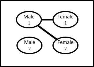
In this network at this time, 50% of men (1 of 2) have concurrent partners, while 0% of women (0 of 2) do. However, the mean number of ties for men (1 per man, averaged from 2 ties for male 1 and 0 ties for male 2) equals the mean number of ties per woman (1 per woman, averaged from 1 tie for female 1 and 1 tie for female 2).
Although the different versions of the model will differ in the level of concurrency, they will have the same overall number of sexual partnerships occurring, the same mean duration for relationships, and the same number of coital acts.
Because this model includes more specific information about the absolute time at which events occur, we can and will make use of information about how the probability of transmission changes as a function of the amount of time the transmitting partner has been infected. That is, we will bring in the “acute infectivity” effect that we explored in Exercise 1. We will use estimates for HIV specifically, drawn from Hollingsworth et al. (2008), which are based on Ugandan serodiscordant couple data (Wawer et al. 2005). These estimates are calculated as monthly transmission probabilities, so each time step in our model will represent a month.
Some aspects of our model are realistic, and others are not. Remember, our goal is to isolate the effect of concurrency, while keeping the model as simple as possible for researchers who are relatively new to modeling. Those who find the insights they gain from these exercises to be provocative are encouraged to learn more about modeling so that they can read both the modeling and the empirical literatures on concurrency with deeper understanding.
Code
The R code for this exercise is printed below. Use the copy button at the top right of the code block to copy it, and paste it into a fresh .R file in your working directory (type getwd() to confirm this location). You can then run the code line by line, or run the entire simulation at once by typing
source("concurrency_exercise_4.R")(or whatever you named the file when you saved it).
Note that when you run the full set of code, it may take 10-15 seconds at the end before your output appears; simulation takes time.
The model as currently set will simulate a population in which concurrency is not allowed for either sex; relationships last a mean of 10 months; the average person is in 0.8 relationships at any time; and initial prevalence is 2%. We suggest:
- First run the model as is, and note the levels of prevalence that emerge.
- Change the two lines at the top about enforcing monogamy from T to F, and rerun.
- Try changing one line to F and one line to T and rerun. Try the reverse.
- Play around with other parameters, like the mean degree, or the initial number of infected people, or the mean relational duration. This allows one to see how general the patterns initially observed are.
- At some point, try stepping through the code line by line, so as to really get a sense of what is happening at each point. Feel free to query different objects as you go to see what they equal, in order to increase your intuition. Because of the time loop in the code, you may want to replace the loop with a single time step so you can run each line in the loop independently.
An additional option is to use the interactive web app that hides the code in the background, and simplifies the process of exploring multiple scenarios. One may use this in addition to, or instead of, working with the code directly. This also allows the scenarios to begin with lower prevalence (1%) than the code does by default, and demonstrate that the equilibrium prevalence is still the same. A third option is to explore the code using the R package concurrency.sim.
####################################
# Parameters
####################################

# Should we enforce a rule of female monogamy?
force.feml.monog <- T
# Should we enforce a rule of male monogamy?
force.male.monog <- T

# Number of females
n.femls <- 5000
# Number of males
n.males <- 5000
# Mean degree (average number of relationships a person has at any one time)
expected.meandeg <- 0.8
# Mean duration of a relationship (in months)
avg.duration <- 10
# Length of the simulation (in months)
numtimesteps <- 1200
# How many females are infected at the start of the simulation?
init.number.of.infected.femls <- 100
# How many males are infected at the start of the simulation?
init.number.of.infected.males <- 100

# Probability of transmission per month for an active relationship,
# from Hollingsworth et al. 2008
beta.by.time.since.inf <- c(rep(0.2055, 3), rep(0.0088, 100),
                            rep(0.0614, 9), rep(0, 10))

####################################
# Basic calculations and book-keeping
####################################

# Total population size
n.pop <- n.femls + n.males
# Expected number of relationships ("edges") in the population at any one time
expected.edges <- round(expected.meandeg * (n.pop) / 2)
# Per-step probability of dissolution for an existing relationship
prob.dissolution <- 1 / avg.duration
# Length of time from HIV infection until death (in months)
time.of.aids.death <- length(beta.by.time.since.inf)
# Cumulative number of female AIDS deaths
cum.num.feml.aids.deaths <- 0
# Cumulative number of male AIDS deaths
cum.num.male.aids.deaths <- 0

# Vectors to store female and male prevalence at each time step
feml.prev <- vector()
male.prev <- vector()

####################################
# Creating the female data frame
####################################

# One row per female
femls <- data.frame(row.names = 1:n.femls)
# HIV status, with everyone starting uninfected (0) for now
femls$hiv.status <- rep(0, n.femls)
# Infection time, unknown (NA) for now
femls$inf.time <- NA
if (init.number.of.infected.femls > 0) {
  # Sample the initially infected females
  init.inf.f <- sample(1:n.femls, init.number.of.infected.femls)
  # Give them infection
  femls$hiv.status[init.inf.f] <- 1
  # Sample their infection times, backdated from the present
  init.inf.time.f <- sample(0:(-time.of.aids.death + 2),
                            init.number.of.infected.femls, replace = TRUE)
  femls$inf.time[init.inf.f] <- init.inf.time.f
}

####################################
# Male data frame
####################################

# All parallel to the female data frame above
males <- data.frame(row.names = 1:n.males)
males$hiv.status <- 0
males$inf.time <- NA
if (init.number.of.infected.males > 0) {
  init.inf.m <- sample(1:n.males, init.number.of.infected.males)
  males$hiv.status[init.inf.m] <- 1
  init.inf.time.m <- sample(0:(-time.of.aids.death + 2),
                            init.number.of.infected.males, replace = TRUE)
  males$inf.time[init.inf.m] <- init.inf.time.m
}

####################################
# Initial contact network
####################################

# A data frame to hold the IDs of the relationship pairs
edgelist <- data.frame(row.names = 1:expected.edges)
# Assign the female side of each edge. Sampling with replacement lets a woman
# appear in several edges (concurrency); without replacement caps her at one
# (monogamy).
if (force.feml.monog == FALSE) {
  edgelist$f <- sample(1:n.femls, expected.edges, replace = T)
} else {
  edgelist$f <- sample(1:n.femls, expected.edges, replace = F)
}
# Same for the male side of each edge
if (force.male.monog == FALSE) {
  edgelist$m <- sample(1:n.males, expected.edges, replace = T)
} else {
  edgelist$m <- sample(1:n.males, expected.edges, replace = F)
}

# A quick check: tabulate relationships per person. When monogamy is enforced
# for a sex, its table is limited to 0's and 1's; otherwise it is not.
table(tabulate(edgelist$f))
table(tabulate(edgelist$m))

####################################
# Time loop
####################################
# Everything above was set-up. This loop is the core of the simulation: at each
# time step we simulate transmission, vital dynamics, and relational dynamics.

for (time in 1:numtimesteps) {

  # --- Transmissions ---

  # HIV status of the female and male partner in each relationship
  hiv.status.feml.partners <- femls$hiv.status[edgelist$f]
  hiv.status.male.partners <- males$hiv.status[edgelist$m]

  # Relationships that are serodiscordant with a positive female (SDPF)
  sdpf <- which(hiv.status.male.partners == 0 &
                  hiv.status.feml.partners == 1)
  # The females in those relationships, and how long they have been infected
  f.in.sdpf <- edgelist$f[sdpf]
  inf.time.sdpf <- time - femls$inf.time[f.in.sdpf]
  # Transmission probability, based on time since the female was infected
  prob.trans.sdpf <- beta.by.time.since.inf[inf.time.sdpf]
  # Flip a weighted coin for each relationship to see if transmission occurs
  trans.sdpf <- rbinom(length(sdpf), 1, prob.trans.sdpf)
  # The newly infected males (double-indexing gets their IDs in one step)
  newly.inf.males <- edgelist$m[sdpf[trans.sdpf == 1]]
  males$hiv.status[newly.inf.males] <- 1
  males$inf.time[newly.inf.males] <- time

  # All parallel for serodiscordant with a positive male (SDPM)
  sdpm <- which(hiv.status.feml.partners == 0 &
                  hiv.status.male.partners == 1)
  m.in.sdpm <- edgelist$m[sdpm]
  inf.time.sdpm <- time - males$inf.time[m.in.sdpm]
  prob.trans.sdpm <- beta.by.time.since.inf[inf.time.sdpm]
  trans.sdpm <- rbinom(length(sdpm), 1, prob.trans.sdpm)
  newly.inf.femls <- edgelist$f[sdpm[trans.sdpm == 1]]
  femls$hiv.status[newly.inf.femls] <- 1
  femls$inf.time[newly.inf.femls] <- time

  # --- Deaths to AIDS ---

  # Who has been HIV positive long enough to die of AIDS?
  femls.dying.of.AIDS <- which(time - femls$inf.time == time.of.aids.death)
  males.dying.of.AIDS <- which(time - males$inf.time == time.of.aids.death)
  # Add the newly dying to the cumulative death counts
  cum.num.feml.aids.deaths <- cum.num.feml.aids.deaths + length(femls.dying.of.AIDS)
  cum.num.male.aids.deaths <- cum.num.male.aids.deaths + length(males.dying.of.AIDS)

  # --- End of ties because of death ---

  # Relationships involving someone who just died, removed from the edgelist
  edges.with.feml.dying.of.aids <- which(edgelist$f %in% femls.dying.of.AIDS)
  edges.with.male.dying.of.aids <- which(edgelist$m %in% males.dying.of.AIDS)
  edges.with.either.dying.of.aids <- c(edges.with.feml.dying.of.aids, edges.with.male.dying.of.aids)
  if (length(edges.with.either.dying.of.aids > 0)) {
    edgelist <- edgelist[-edges.with.either.dying.of.aids, ]
  }

  # --- End of other ties randomly ---

  # Flip a weighted coin for each remaining relationship, and break the winners
  edges.coinflip <- rbinom(dim(edgelist)[1], 1, prob.dissolution)
  edges.to.break <- which(edges.coinflip == 1)
  if (length(edges.to.break > 0)) {
    edgelist <- edgelist[-edges.to.break, ]
  }

  # --- Add new edges ---

  # Add as many new edges as were lost, keeping the edge count fixed
  num.ties.to.add <- expected.edges - dim(edgelist)[1]
  if (num.ties.to.add > 0) {
    # Draw the female side: with replacement if concurrency is allowed,
    # otherwise from women who currently have no relationship
    if (force.feml.monog == F) {
      f <- sample(1:n.femls, num.ties.to.add, replace = T)
    } else {
      femls.with.no.ties <- setdiff(1:n.femls, edgelist$f)
      f <- sample(femls.with.no.ties, num.ties.to.add, replace = F)
    }
    # Same for the male side
    if (force.male.monog == F) {
      m <- sample(1:n.males, num.ties.to.add, replace = T)
    } else {
      males.with.no.ties <- setdiff(1:n.males, edgelist$m)
      m <- sample(males.with.no.ties, num.ties.to.add, replace = F)
    }
    # Pair the new females and males and bind them onto the edgelist
    new.edges <- data.frame(f, m)
    edgelist <- data.frame(rbind(edgelist, new.edges))
    row.names(edgelist) <- 1:dim(edgelist)[1]
  }

  # --- Insert new births ---

  # Replace each person who died of AIDS with a new, uninfected arrival:
  # reset HIV status to 0 and infection time to NA
  new.feml.ids <- femls.dying.of.AIDS
  femls$hiv.status[new.feml.ids] <- 0
  femls$inf.time[new.feml.ids] <- NA

  # All parallel with males
  new.male.ids <- males.dying.of.AIDS
  males$hiv.status[new.male.ids] <- 0
  males$inf.time[new.male.ids] <- NA

  # --- Track prevalence ---

  # Record current female and male prevalence for this time step
  feml.prev[time] <- mean(femls$hiv.status)
  male.prev[time] <- mean(males$hiv.status)

}

# Set up a two-panel plotting window and plot prevalence over time
windows(20, 10)
par(mfrow = c(1, 2))
plot(feml.prev, main = "Female prevalence over time ", ylim = c(0, 0.5))
plot(male.prev, main = "Male prevalence over time ", ylim = c(0, 0.5))
Discussion
When one runs the code as is, and then turns concurrency on and off, one finds the following HIV prevalences at equilibrium:
| Network model | Prevalence |
|---|---|
| Concurrency allowed for both sexes | about 29% for both sexes |
| Concurrency allowed for one sex but not the other | about 18% for the sex without concurrent partners, and about 15% for the sex with concurrent partners |
| Concurrency not allowed for either sex | about 1% for both sexes |
And, when one follows through all of the detailed logic of the code, one can see for oneself that each model includes the same amount of partnerships and the same number of sexual acts as the others. The only difference is whether concurrency is allowed or not. And this simple fact is the difference between 29% HIV prevalence and 1% HIV prevalence. One also sees, in the cases where one sex could have concurrent partners and the other could not, that not only was there an intermediate-sized epidemic, but the sex that could not have concurrency ended up with the greater prevalence. This matches the fundamental point about how concurrency works that we have been reiterating throughout this tutorial: concurrency leads to higher prevalence in the partners of those with concurrent partners.
Note that these numbers combine all of the different phenomena by which concurrency operates; they result jointly from the effect of backwards transmission (partly offset by reduced forward transmission), acute infectivity, and path acceleration.
Of course this scenario was selected as the default because it presents a dramatic picture. How generalizable is this trend? And what happens at the behavioral values that seem most realistic? As one explores further, one will see that the concurrency simulations always generate larger epidemics than the same scenario without, and that there is a reasonable behavioral range over which one gets a large epidemic with concurrency and none or very little without.
As we stated at the outset, there are various simplifications for this model. The most important one is that concurrency can only be handled in a binary fashion: either the model allows it or doesn’t (within each sex), and when it does allow it, the amount of concurrency is determined by the mean degree alone. There is no way to model different levels or patterns of concurrency for a given number of sexual relations. This is of course an important thing to be able to do—one wants to be able to simulate observed behavioral data, including mean degree and prevalence of concurrency for both men and women, as faithfully as possible to one’s data. That requires a much more sophisticated set of modeling tools than we can provide in an introduction like this, but that is precisely what is done in the concurrency modeling literature. For those interested in learning more about these tools, see the More Resources section.
And of course, there are many other simplifications. This model did not include any coital dilution (the tendency for people in multiple simultaneous relationships to have fewer sex acts per unit time with one or more of their partners than someone in one relationship). We did not model circumcision, or co-infections with STIs, or treatment, or many other things. There was no age structure present. All of those things can be added, making the model more realistic but more difficult for modeling newcomers to understand them. We hope, now that we have developed together some first-hand intuition about concurrency and the magnitude of its potential impact, that readers will be interested in learning more about the theory and methods needed to be able to read that literature in depth. We point to some of the resources for doing so on the More Resources section.
With partnerships, durations, and sex acts held identical, equilibrium prevalence rose from about 1% with no concurrency to about 29% with it. And the sex that could not have concurrent partners ended up with the higher prevalence, the central lesson of the whole tutorial.